Camera Calibration and Lens Distortion

Connect Known And Observed Corners

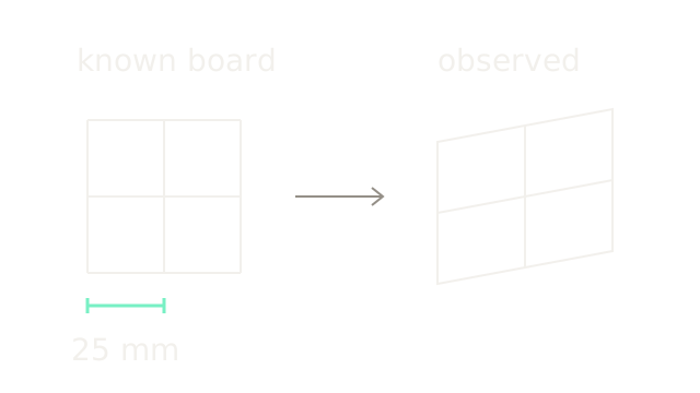
Calibration estimates the camera parameters that make known scene points project to their observed image locations. A measured planar board provides coordinates; multiple images provide different views of them. The result separates shared intrinsics, a pose for each view, and coefficients describing lens distortion. It does not directly measure the depth of an arbitrary new scene.

Our three-by-three board corners have 25 mm spacing. Set the first corner to (0,0,0) meters and the next to (0.025,0,0). The selected interval is 70 drawing units; the image grid is a schematic projective view, not the numerical camera fixture below. Correct units and a flat, rigid board matter. OpenCV's calibration workflow connects known object points to detected image corners.

Scale Rays Into Pixels

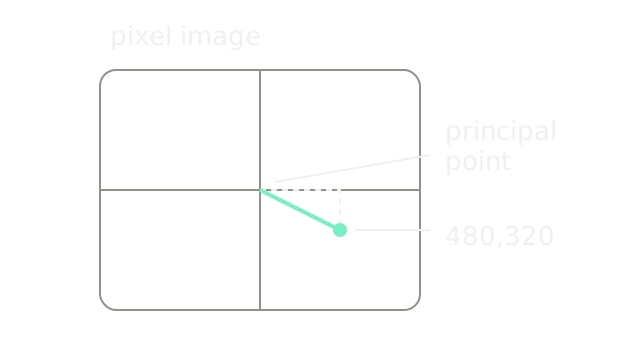
First ignore distortion. A camera-space point (Xc,Yc,Zc) defines normalized coordinates x=Xc/Zc, y=Yc/Zc. For a zero-skew model, u=fx x+cx, v=fy y+cy. Focal lengths fx,fy are in pixels; (cx,cy) is the principal point.

Use fx=fy=800 and (cx,cy)=(320,240). The ray (x,y)=(0.2,0.1) lands at (480,320) pixels because 800×0.2+320=480 and 800×0.1+240=320. The 640×480 image is drawn at half scale. The mint displacement from the principal point is therefore (80,40) drawing units, corresponding to (160,80) pixels. The principal point need not be exactly the image center in a calibrated camera. See OpenCV's projection equations.

Transform The Board Pose

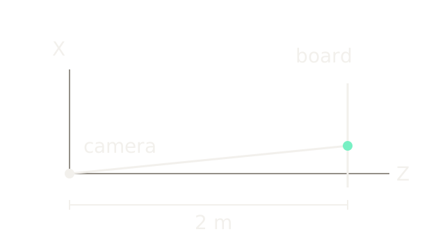
Intrinsics describe the camera; extrinsics describe the board's position and orientation relative to it. The world-to-camera convention is Pc=R Pw+t. In this separate pose example, R=I and t=(0,0,2) meters move board point (0.2,0.1,0) to (0.2,0.1,2). Its normalized ray is (0.1,0.05), so the previous K projects it to (400,280) pixels.

The side view suppresses Y and uses 200 drawing units per meter in X and Z. The board lies at depth 2; the mint point is 0.2 meters off the optical axis. Every calibration image needs its own R and t. Moving the board does not change the camera's focal length under the fixed-camera assumption.

Model Radial Distortion

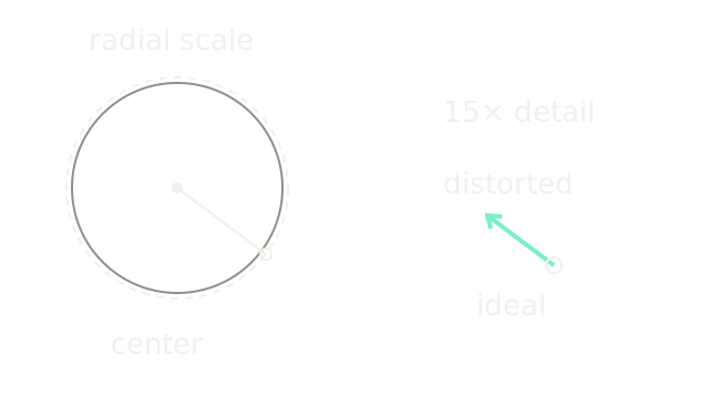
For an isolated first-order example, let r²=x²+y² and multiply both coordinates by 1+k1 r². At (0.4,0.3), r²=0.25. Choose k1=−0.2, giving scale 1−0.2×0.25=0.95 and distorted point (0.38,0.285). These are normalized coordinates, not pixel offsets.

The dashed ideal radius is 100 drawing units; the distorted radius is 95, at 200 units per normalized coordinate. The detail magnifies the displacement 15 times, from (-0.02,-0.015) to (-60,-45) drawing units. Both coordinates use image y downward. Higher-order radial terms can change the behavior away from this example; a single negative coefficient is not a universal lens description.

Add Tangential Offsets

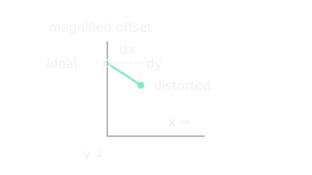
The common model adds tangential terms controlled by p1,p2. Isolate them from radial distortion and reuse (x,y)=(0.4,0.3), r²=0.25, with p1=0.01, p2=0.02:

$$\Delta x=2p_1xy+p_2(r^2+2x^2)=0.0024+0.0114=0.0138,$$ $$\Delta y=p_1(r^2+2y^2)+2p_2xy=0.0043+0.0048=0.0091.$$

The new point is (0.4138,0.3091). The picture magnifies these small changes to 5,000 drawing units per normalized coordinate: 69 right and 45.5 down. It shows a local displacement, not the complete field or a physical lens shift. Radial and tangential terms combine before intrinsics convert to pixels. The five-coefficient model and its equations are specified in the calibration tutorial; wide-angle optics may need a different model.

Vary The Board Orientation

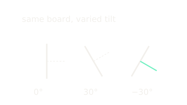
The three side-view board segments have equal length 120 and tilts 0°, 30° and −30° from vertical. Short perpendicular strokes show their normals; position here only separates examples. Tilt changes the projective constraints while the camera intrinsics remain shared. Also cover different image regions to observe distortion away from the center.

Zhang's calibration report, sections 2–4 uses plane-to-image homographies to constrain intrinsics, initializes the camera and poses, then refines them. It identifies degenerate configurations when board orientations do not supply independent information. Collecting many nearly identical frontal images is weaker than collecting varied usable views; an extreme tilt can make corner localization unreliable.

Compare Predictions To Detections

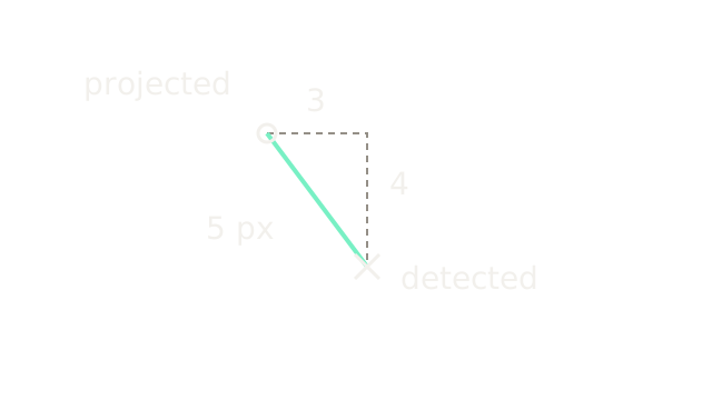
Project a known board point using the candidate intrinsics, pose and distortion. If the model predicts (480,320) pixels while the detected corner is (483,324), the residual is (3,4) and its length is 5 pixels. The hollow circle is the projection; the cross is the measured corner. The magnified image uses 30 drawing units per pixel. This checks one observation, not the quality of a complete calibration. Blurred corners, incorrect correspondences and a warped board can all raise residuals.

Refine Across All Observations

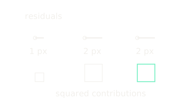
Calibration refinement adjusts shared intrinsics and distortion together with each view's pose to reduce the sum of squared coordinate residuals. For three toy residual lengths [1,2,2] pixels, the squared contributions are [1,4,4] square pixels, totaling 9. Their per-point root mean square is sqrt(9/3)=sqrt(3)≈1.732 pixels. Dividing by six scalar coordinates instead would define a different statistic; state the convention.

The upper line lengths use 30 drawing units per pixel; lower square areas encode the squared contributions, with sides 30, 60 and 60. These are objective contributions at one candidate solution, not a fabricated optimizer trace. Check residual patterns by image region and validate on additional views. A small training residual alone cannot establish accurate physical parameters.

Resample An Ideal Output

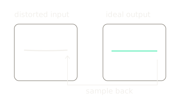
For each ideal output location, use the lens model to find its donor coordinate in the distorted input. Thus the output ray (0.4,0.3) looks up (0.38,0.285) under our radial-only example. This is backward raster sampling even though the distortion equation maps ideal coordinates forward into distorted ones.

The ideal row y=0.3, x∈[−0.4,0.4] is straight on the right. In the distorted input, its endpoints have y 0.285 and its center y 0.2946, producing the shallow curved row on the left. Both views use 200 drawing units per normalized coordinate; the cubic's controls come from that model, not an arbitrary bow. The reverse-lookup connector uses a lower lane. Inverse sampling also explains interpolation and border choices. Correction may leave invalid borders or crop the field of view; it does not recover lost source detail.

Where It Breaks

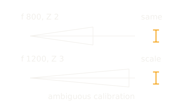
With a frontoparallel board, image spacing depends on the ratio f/Z. Both (f,Z)=(800 px,2 m) and (1200 px,3 m) give 400 pixels per meter. A 25 mm board interval therefore projects to ten pixels in either configuration. The amber intervals show this identical observation even though the inferred camera differs.

The side-view depth scale is 110 drawing units per meter; board height uses a separate 300 units per meter to keep the ray geometry readable. The amber image intervals use four drawing units per pixel. These separate axes are schematic, not a drawing of the physical focal plane. One frontal view cannot separate these quantities without additional information. Repeated parallel poses can preserve degeneracies, and central-only coverage weakly constrains edge distortion. Change board orientation, cover the field, choose an appropriate lens model, and validate held-out projections. Recalibrate or transform intrinsics appropriately when zoom, focus, crop or image scaling changes.

The Quick Version

• Measured board spacing supplies known physical coordinates.
• Intrinsics scale normalized rays and locate the principal point.
• Extrinsics transform board coordinates into each camera view.
• Radial distortion scales coordinates according to distance from center.
• Tangential terms add direction-dependent coordinate offsets.
• Varied board orientations constrain shared intrinsics more independently.
• Reprojection residuals compare projected and detected image locations.
• Joint refinement minimizes squared residuals across observations.
• Undistortion samples distorted input for an ideal output grid.
• Frontoparallel scale ambiguity can hide behind a low residual.