Homography and Image Stitching

Find Shared Scene Evidence

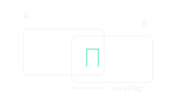
A homography is a projective map between two image planes. It aligns views of one scene plane; pure rotation about a camera's projection center also permits a homography for arbitrary scene depth. Stitching uses that map to place overlapping images on a common canvas, then manages brightness and source ownership. The OpenCV homography reference derives these cases.

Here two 200-unit-wide crops are offset by 120 scene units, sharing 80. At 1.4 drawing units per scene unit, widths are 280 and overlap is 112. The outline of B is lowered 25 drawing units only to distinguish the crops. The shared mint landmark is the evidence, not a blended output. Feature matching and RANSAC explains how to obtain candidate correspondences and reject inconsistent ones.

Divide Homogeneous Coordinates

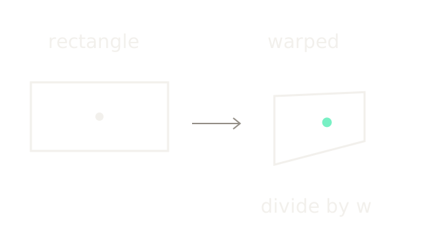
Use the synthetic map below, with pixel coordinates x right and y down:

$$H=\begin{bmatrix}1&0&40\\0&1&20\\0.002&0&1\end{bmatrix},\quad x'=\frac{x+40}{1+0.002x},\qquad y'=\frac{y+20}{1+0.002x}.$$

At (100,50), the homogeneous result is (140,70,1.2), so the mint point is (116.667,58.333). Ignoring the final division would produce a different transformation. Both panels use one drawing unit per pixel, with separate origins. The same rectangle changes width and height with position. Multiplying every matrix entry by any nonzero scalar preserves the map; there are eight independent parameters. Locations where the denominator vanishes cannot be drawn as finite pixels.

Constrain The Plane Map

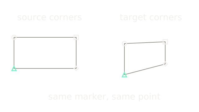
Track marker identity between the panels. Source corners (0,0),(200,0),(200,100),(0,100) map to (40,20),(171.429,14.286),(171.429,85.714),(40,120). Each pair supplies two coordinate constraints. Four pairs in general position can constrain the eight freedoms; collinear configurations cannot. Noisy data needs additional, spatially distributed correspondences and robust estimation. The previous beat's mint center was a test point; these four corners are the estimation constraints.

Preserve Lines, Change Parallels

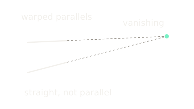
The solid segments are the transformed top and bottom edges from the same fixture. Their dashed extensions meet at (500,0) in target coordinates. To check it, the source horizontal point at infinity (1,0,0) maps through H to (1,0,0.002), which divides to (500,0,1). The display origin is now (50,120), so the meeting point appears at (550,120). Lines stay straight, but parallelism and lengths are not generally preserved. This separates a projective map from an affine one.

Sample Backward From Output

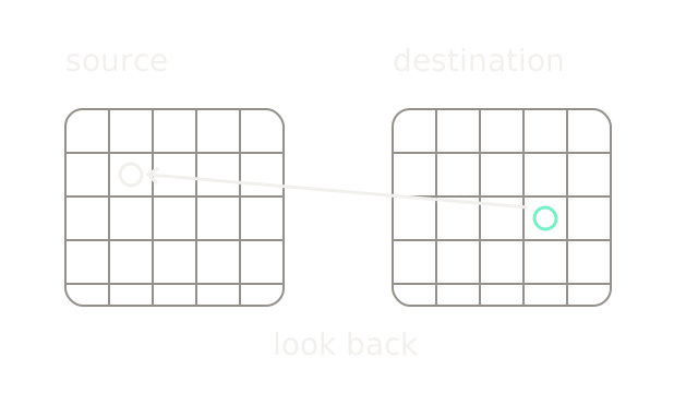
Knowing where source points move is not enough to fill a raster. Forward-moving integer samples can leave output gaps. Instead visit each destination pixel, apply the inverse map, and sample the source there. For this separate translation example, H:(x,y)→(x+40,y+20), destination (70,50) looks up source (30,30). The backward arrow intentionally crosses the sampling grids to connect those locations. Each panel uses two drawing units per pixel. OpenCV's geometric transformation documentation specifies destination-to-source sampling and border handling. An inverse flag changes how the supplied matrix is interpreted; it does not change the need to sample every destination location.

Interpolate Fractional Samples

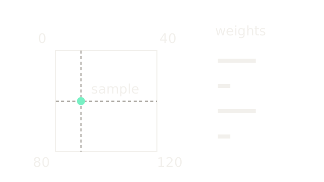
Inverse coordinates usually fall between source samples. Zoom into a unit square with values top-left 0, top-right 40, bottom-left 80 and bottom-right 120. The mint location is (0.25,0.5) within it. Bilinear weights in that order are 0.75×0.5=0.375, 0.25×0.5=0.125, 0.375, and 0.125. Their sum is 1. The four bars on the right show those weights in the same order at 200 drawing units per weight unit.

The interpolated value is 0.375×0 + 0.125×40 + 0.375×80 + 0.125×120 = 50. Interpolation estimates between stored values; it cannot recover detail absent from the source, and repeated resampling can blur it.

Allocate The Combined Canvas

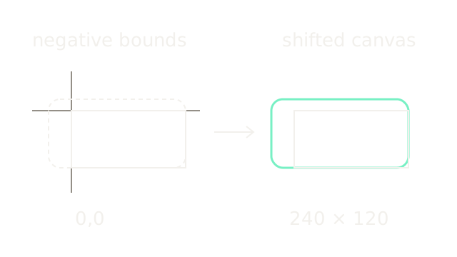
Transform image corners and include both images when computing output bounds. In this separate canvas fixture, combined extents are x∈[−40,200], y∈[−20,100], shown at 0.8 drawing units per coordinate unit. Shift the combined frame by (40,20) to obtain nonnegative coordinates and a continuous extent of 240×120. The inner rectangle is the unwarped reference image; its position relative to the enlarged bounds remains fixed. Axes cross at the old origin on the left.

Compose this canvas translation after the image warp: Hcanvas = T H. Actual raster allocation uses a stated pixel-center convention and rounded bounds. Large projective extents or a horizon crossing require a crop or different projection rather than unlimited allocation.

Compensate For Exposure

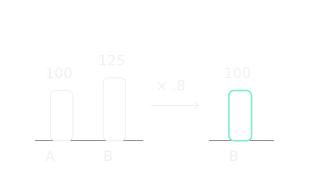
Aligned pixels can still disagree in intensity. Suppose a stable overlap region has value 100 in A and 125 in B. A scalar gain 100/125=0.8 maps B to 100. All three bars share one drawing unit per intensity unit. This toy gain assumes a consistent multiplicative relationship without clipping. It cannot remove local shadows, vignetting or response nonlinearities by itself. Geometry and photometry are distinct problems; a better homography does not fix exposure.

Choose A Seam And Blend

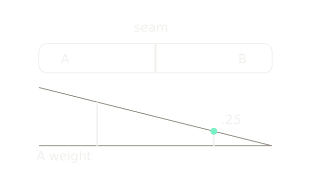
The top strip shows a hard ownership boundary: use A on one side and B on the other. The lower profile instead decreases A's mixing weight across an overlap, from 1 to 0. Its height is 120α drawing units; the mint point has α=0.25, so B receives 0.75. For another toy pair IA=100, IB=120, the blend is 0.25×100+0.75×120=115. A seam and a feathered blend solve different parts of compositing. This linear illustration is not a complete multiband panorama algorithm. Mixing misaligned edges still produces ghosting.

Where It Breaks

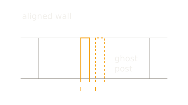
For a rectified horizontal translation, use focal length 200 pixels and baseline 0.2 meters. A post at 2 meters shifts 200×0.2/2=20 pixels, while a wall at 4 meters shifts 10. Aligning the wall leaves a ten-pixel post mismatch, drawn as 50 units at five units per pixel. Solid and dashed outlines identify the two warped views of the same foreground post.

A single plane map cannot remove these depth-dependent shifts. Blending may soften the double edge but cannot make both projections geometrically correct. Pure camera rotation avoids this translational parallax; moving objects, lens distortion and rolling shutter can introduce other alignment failures. Stereo depth turns depth-dependent displacement into a measurement instead.

The Quick Version

• Overlap supplies common scene evidence for alignment.
• Homography coordinates require division by their homogeneous scale.
• Four general-position point pairs constrain eight independent parameters.
• Straight lines stay straight; parallelism need not survive.
• Inverse warping samples the source for each output pixel.
• Bilinear interpolation combines four neighboring source values.
• Canvas translation retains warped content with negative coordinates.
• Exposure compensation addresses brightness differences after alignment.
• Seams select ownership; blending mixes source values.
• Translational parallax prevents one homography from aligning arbitrary depths.