Convolutional Neural Networks for Images

Start With Local Evidence

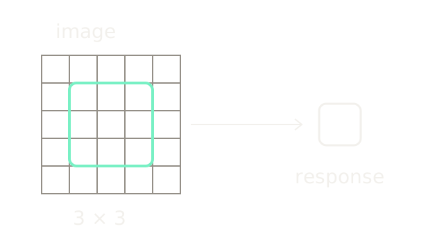
A convolutional neural network (CNN) learns filters that turn local image measurements into spatial feature maps. It combines those responses through nonlinear layers and aggregation to make predictions. The highlighted 3×3 window is the support for one response in a 5×5 input.

Locality reduces connections compared with a fully connected image layer. It also limits what a single early response can know. For the general network pipeline, see the core CNN visual; this page examines its image operations.

Compute A Filter Response

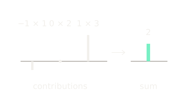
This one-dimensional slice isolates the arithmetic. Pixels [1,2,3] and weights [−1,0,1] give contributions [−1,0,3], summing to 2 with zero bias. The common stem scale encodes signed contributions and the output. The negative contribution extends below zero.

Deep-learning “convolution” usually computes cross-correlation without flipping the kernel. A 2D filter repeats this multiplication across both spatial dimensions. Its weights are learned from a loss, rather than fixed as in a conventional image filter.

Reuse The Same Weights

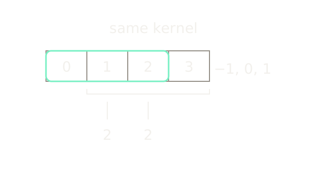
Slide [−1,0,1] over [0,1,2,3]. The first window gives −0+2=2; the second gives −1+3=2. The outline selects the first window and the bracket selects the next. The kernel stays fixed during this forward pass.

Weight sharing makes a filter detect the same local pattern at many locations without learning an independent copy per location. It does not make the entire classifier invariant to every translation. Padding, boundaries, stride and later layers matter.

Sum Across Channels

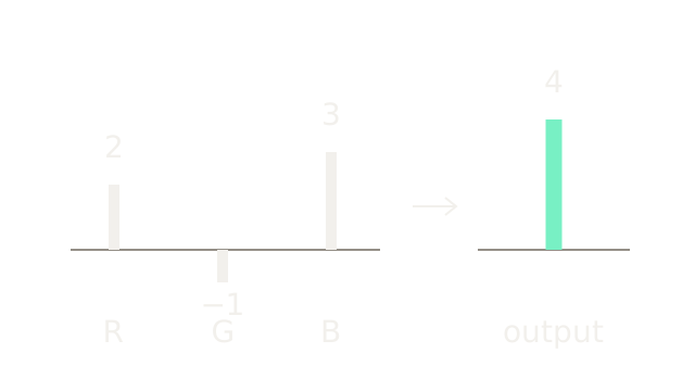
For an RGB input, one ordinary convolution filter has a spatial kernel for each input channel. The R, G and B labels identify channels without using channel colors. Their illustrative dot products 2,−1,3 combine into 2−1+3=4 before bias and activation.

A 3×3 RGB filter has 3×3×3=27 weights. Adding one bias gives 28 parameters; two independent output filters require 56. Output channels count different learned filters, not separate red, green and blue images. The pictured channel contributions are a separate fixture from the preceding single-channel slice.

Gate Negative Responses

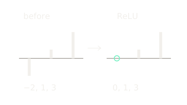
ReLU applies max(0,z) to each response. The vector [−2,1,3] becomes [0,1,3] on the same amplitude scale. The outlined zero marks the gated negative value. A zero-bias stack of linear filters would still be linear without nonlinear operations.

ReLU's derivative is zero on negative inputs, so a persistently inactive unit can stop receiving useful local gradient. This drawing demonstrates the forward gate; it does not claim every CNN uses ReLU.

Choose The Sampling Step

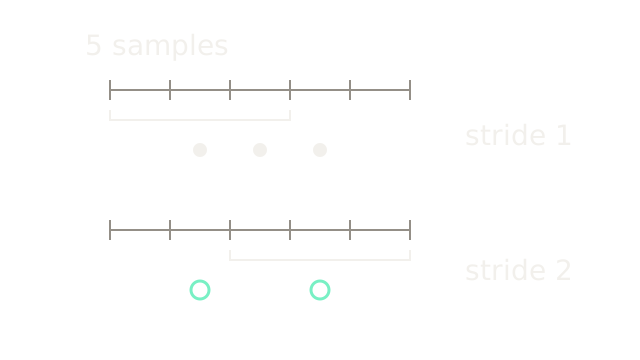
For input length N, kernel width K, padding P and stride S, output length is floor((N+2P−K)/S)+1. Here N=5, K=3 and P=0. Stride 1 gives three valid centers; stride 2 gives two. Brackets identify example window supports; dots identify evaluated centers.

Apply the same rule separately to image height and width. Padding can retain a chosen spatial size, but it introduces a boundary convention. Stride reduces computation and feature resolution while potentially discarding detail. Stanford's CNN notes describe these layer shapes and parameter sharing.

Keep A Local Maximum

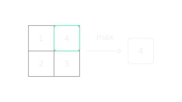
The 2×2 response window [1,4;2,3] reduces to 4. The selected cell and output share the same value; the output does not record which of the four positions supplied it. Pooling is a fixed aggregation, not a learned convolution kernel.

Keeping a strong response can tolerate some movement inside a window, but window boundaries still matter. Max pooling and strided convolution both reduce resolution; neither automatically guarantees translation invariance.

Grow The Receptive Field

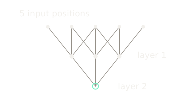
Each first-layer node reads three adjacent inputs. The selected second-layer node reads three first-layer nodes, whose support union covers all five original inputs. Crossings are independent dependency edges; only dots are nodes.

For stride 1, two width-3 layers give receptive width 1+(3−1)+(3−1)=5. Two 3×3 layers similarly cover a 5×5 theoretical spatial field. This is possible influence, not a claim that all inputs receive equal learned weight. Larger support helps combine local parts, at the cost of more operations and intermediate activations.

Pool Before Classification

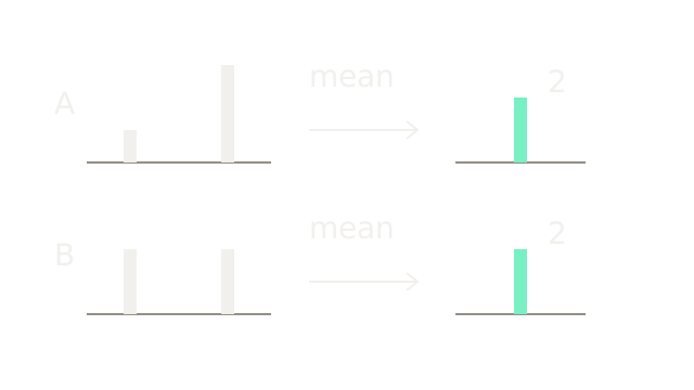
Global average pooling summarizes each channel over its spatial locations. In this two-position example, channel A has values [1,3] and B has [2,2]. Both means are 2. A classifier can then combine pooled channel values into class scores.

The equal outputs show information loss: a concentrated response and a uniform response can have the same mean. A classification head may suit “what is present”; localization needs retained spatial evidence. These are feature responses, not class probabilities.

Where It Breaks

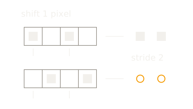
Consider a periodic row [1,0,1,0] and its one-position shift [0,1,0,1]. A stride-2 identity filter samples indices 0 and 2. The outputs change from [1,1] to [0,0], shown by solid squares versus amber empty rings. Empty input cells encode zero.

This is an exact counterexample to claiming that shared convolutions make the full network shift-invariant. Anti-alias filtering and suitable augmentation can reduce sensitivity, with a detail or training trade-off. For pixel-accurate tasks, use architectures that preserve or recover spatial resolution rather than relying solely on a pooled classifier.

The Quick Version

• Local kernels read image neighborhoods.
• Weighted pixel contributions sum into filter responses.
• Shared weights reuse one detector across spatial positions.
• Each output filter aggregates across input channels.
• ReLU gates negative responses.
• Stride and padding determine output resolution.
• Max pooling retains strength while discarding exact local position.
• Stacked filters expand theoretical receptive fields.
• Spatial averaging summarizes each channel before classification.
• Strided sampling can amplify sensitivity to a one-pixel shift.