Image Classification Architectures, LeNet to ResNet

From Image To Class

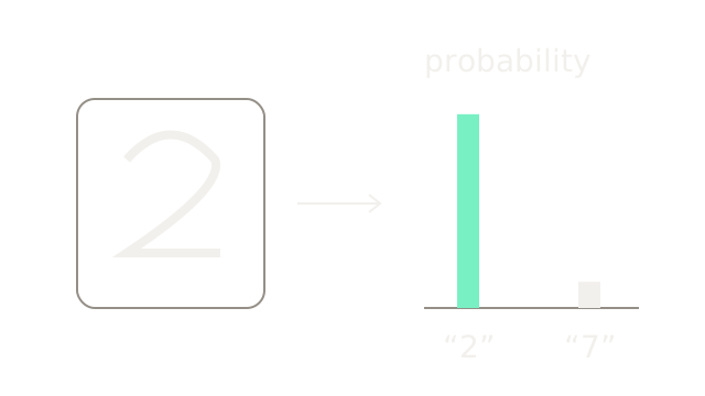
An image classifier combines spatial features into scores for image-level categories. LeNet, AlexNet, VGG, Inception and ResNet change how those features are extracted, reduced and trained. Their design choices solve different constraints; depth alone is not a selection rule.

The digit sketch feeds a toy two-class softmax with logits [2,0]: e²/(e²+1)=0.8808 for “2” and 1/(e²+1)=0.1192 for “7”. The stems are proportional to these probabilities, not predictions measured from any historical model. For local operations, start with CNN image mechanics.

LeNet Shrinks Spatial Maps

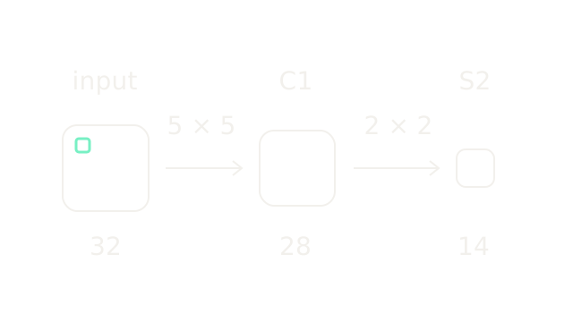
This detail follows the first stages of LeNet-5, section II. A 32×32 input with a valid 5×5 convolution becomes a 28×28 feature map: 32−5+1=28. Subsampling with 2×2 groups reduces each side to 14. Square side lengths share one pixel scale.

C1 and S2 each have six maps; the drawing shows one representative footprint per stage, not the full architecture. LeNet's subsampling sums local inputs, applies a learned coefficient and bias, then a nonlinear function. It is not the modern fixed max-pooling operation. Lower resolution reduces work while sacrificing fine position.

AlexNet Uses Non-saturating Activation

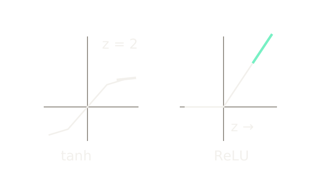
AlexNet's section 3.1 compares ReLU with saturating activations. The two plots share input and output scales. At input z=2, tanh(2)=0.9640 with derivative 1−tanh²(2)=0.07065; ReLU outputs 2 with derivative 1. Short thick tangents expose the slope difference; thin connected samples guide the activation shape.

This is a local derivative comparison, not a training-speed measurement. AlexNet also combined convolution, pooling, GPU computation, augmentation and dropout. ReLU can block gradient on its negative side, so activation choice alone does not solve optimization.

VGG Stacks Small Kernels

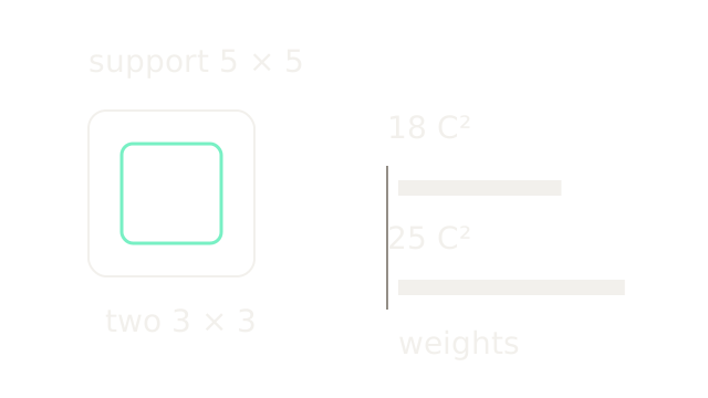
Two stride-1 3×3 layers cover a 5×5 theoretical input field. With C input, intermediate and output channels, they use 2×9C²=18C² weights versus 25C² for one 5×5 layer, omitting biases. At C=64 this is 73,728 versus 102,400; the bars share one parameter scale.

VGG's architecture discussion motivates stacking small filters. The inner outline is a 3×3 support within the larger 5×5 union, not the entire two-layer computation. An intermediate nonlinearity makes the stack functionally different from one linear large kernel. More layers also require stored activations and computation.

Inception Combines Parallel Scales

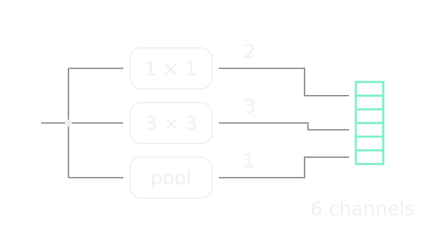
Inception processes a shared input through parallel branches and concatenates the results along channels. The illustrated subset uses output channel counts 2, 3 and 1, yielding 2+3+1=6 channels. Each output strip is one channel; the spatial height and width must agree for concatenation.

This simplified subset omits the 5×5 branch and internal reductions from the original Inception module. The pooling branch includes a projection producing its stated one channel. Concatenation retains branch outputs separately; it is not elementwise addition.

Reduce Before Expensive Filtering

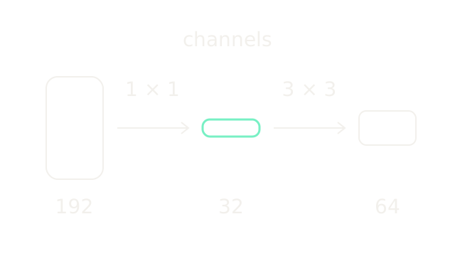
A 1×1 layer can mix channels at each position while reducing their count. This toy detail reduces 192 channels to 32, then uses a 3×3 convolution to produce 64. Band height encodes channel count, with spatial dimensions held fixed.

The reduction uses 192×32=6,144 weights; the spatial layer uses 9×32×64=18,432. Total 24,576 is below the direct 9×192×64=110,592. These counts exclude biases, normalization and other branches. Compression can discard useful information; parameter reduction is not an accuracy guarantee.

ResNet Learns A Correction

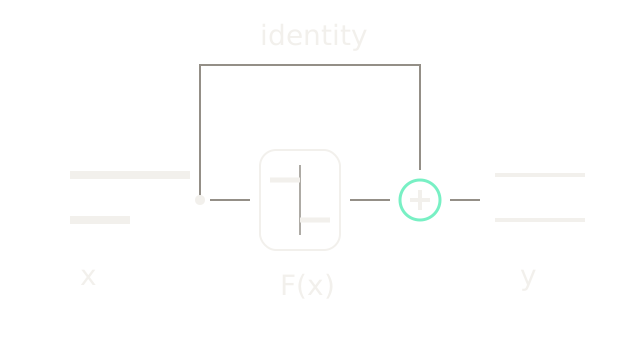
Plain depth can make training harder. A residual block instead computes y=x+F(x): the upper bypass carries x around the learned branch, and the plus combines corresponding components. Here x=[2,1], F(x)=[−0.5,0.5], so y=[1.5,1.5]. Horizontal lengths encode magnitude; the correction's vertical reference separates negative from positive components.

This is the pre-activation-output detail; the original ResNet block applies ReLU after addition. An identity shortcut adds no learned weights and supplies a direct derivative term. It helps optimization without guaranteeing that every deeper model trains better.

Match The Shortcut Shape

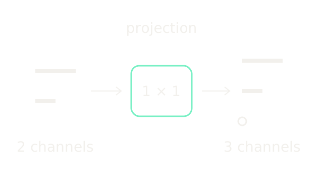
Elementwise addition requires matching spatial and channel dimensions. A projection shortcut can transform x before addition when the branch changes shape. The toy matrix [[1,0],[0,1],[0,0]] maps [2,1] to [2,1,0], making three channels. The empty ring identifies the added zero-valued component.

A learned 1×1 projection can use other values; zero padding is merely this fixture's numerical result. Downsampling blocks also need compatible spatial reduction. Projection costs parameters, unlike a same-shape identity shortcut.

Narrow The Spatial Work

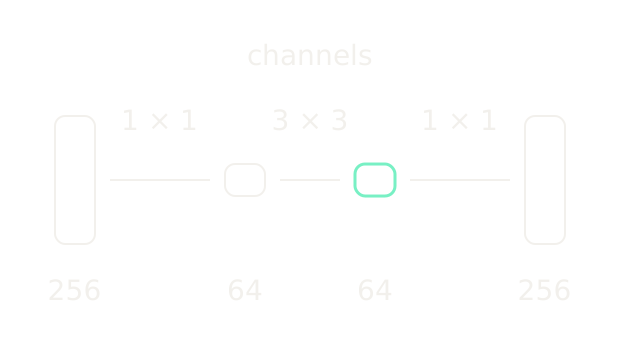
The bottleneck detail changes channels 256→64→64→256 using 1×1, 3×3 and 1×1 layers. All band heights share one channel scale. The 3×3 operation works between narrow representations, then the last layer restores the width needed for addition to the identity path.

At unchanged resolution, weight count is 256×64+9×64×64+64×256=69,632, excluding biases and normalization. The shortcut and addition are omitted here because the previous beats explain them. Reducing the middle width controls spatial cost, but also constrains the representation.

Where It Breaks

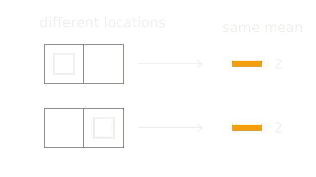
Feature maps [4,0] and [0,4] place the same response at different locations. Global averaging yields 2 for both. A classifier that receives only that pooled value cannot recover which location supplied it, regardless of how deep the backbone is.

This is a precise counterexample for the depicted pooling operation, not a claim that every full network produces identical features for shifted images. Image classification is the wrong output contract when the goal is several object boxes or a pixel mask. Keep spatial predictions for object detection or segmentation, and select architecture using the task, resolution, memory and training data.

The Quick Version

• Classification maps image evidence to class scores.
• LeNet alternates convolution and spatial subsampling.
• ReLU preserves positive slopes where tanh can saturate.
• Stacked small kernels expand support with fewer equal-width weights.
• Inception concatenates features from parallel branches.
• Channel reduction lowers subsequent spatial-convolution cost.
• Residual blocks add learned corrections to identity paths.
• Projection shortcuts match dimensions before addition.
• Bottlenecks concentrate spatial computation in narrow channels.
• Global classification pooling can erase location information.