Visual explainer
Feature Descriptors with SIFT and ORB
Describe local patches with SIFT gradient histograms or ORB binary comparisons, align their scale and orientation, and see why repeated patterns remain ambiguous.
Describe The Patch
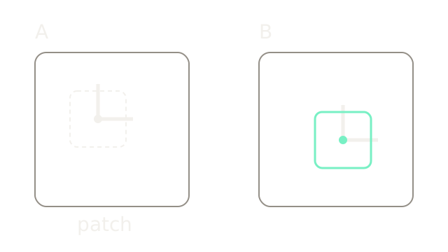
A detector chooses where to look; a descriptor encodes what the neighborhood looks like so another image can be searched for similar evidence. SIFT uses local gradient histograms; ORB uses binary intensity comparisons. The same L appears at different coordinates in A and B, so coordinates alone cannot connect it. The outlined crops select surrounding evidence, not physical object boundaries. Start with corner detection for the location-selection problem.
Follow The Feature Scale
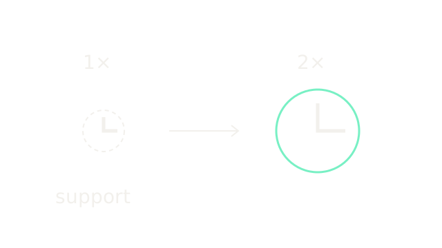
Doubling the L's size doubles the illustrative support radius from 30 to 60 drawing units. A fixed crop would see different fractions of the motif. SIFT detects extrema across scale space and describes at the selected scale; ORB detects features on an image pyramid. This schematic shows corresponding support, not either detector's exact sampling footprint. Discrete scales and resampling limit repeatability.
Align The Local Frame
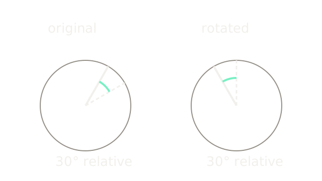
The dashed ray is the assigned frame; the solid ray is a gradient. Here angles use mathematical y upward. Initially the gradient is 60° and the frame 30°: the relative angle is 30°. Rotate both by 60° and it remains 120°−90°=30°. SIFT assigns orientation from nearby gradients and expresses its descriptor relative to that frame. Multiple strong orientation peaks may produce multiple oriented keypoints. This ideal calculation does not guarantee identical descriptors after raster rotation.
Pool Gradient Evidence
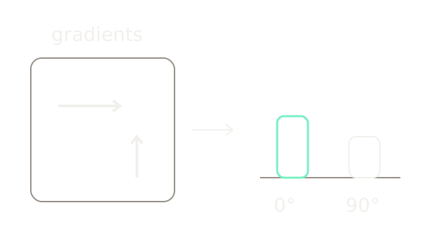
Isolate two gradients (3,0) and (0,2) in one cell. Their magnitudes are 3 and 2; their directions are 0° and 90°. With unit weights, they contribute 3 and 2 to those bins. Both arrows and bars use 30 drawing units per magnitude unit. Actual SIFT adds spatial Gaussian weighting and interpolation across neighboring spatial and orientation bins; this picture isolates pooling rather than reproducing those weights.
Keep Rough Spatial Arrangement
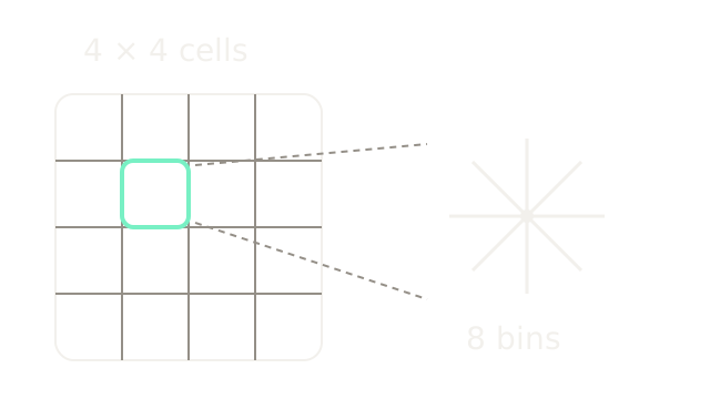
A single histogram forgets where each edge lies. SIFT retains a coarse arrangement using a four-by-four array of cells, each with eight orientation bins: 4×4×8=128 components. The selected cell is enlarged on the right; its spokes identify eight bin directions, with equal illustrative lengths rather than measured magnitudes. The dashed leaders indicate magnification and intentionally pass across the parent grid. Concatenating the cell histograms preserves rough position while tolerating small local shifts. Lowe's paper, section 6 gives the descriptor construction.
Reduce Contrast Sensitivity
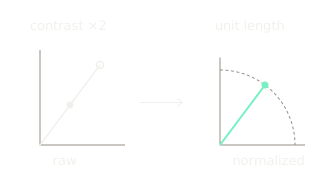
For a toy two-component vector, ||(3,4)||=5, giving (0.6,0.8). Doubling positive contrast gives (6,8) with norm 10 and the same normalized vector. The left plot uses 20 drawing units per raw component; the right deliberately zooms to 150 per normalized component. Its dashed quarter-circle is the unit-length boundary. This demonstrates normalization only. SIFT also clips normalized components at 0.2 and renormalizes to reduce dominance by large gradients. That threshold applies to the full descriptor, not this two-component teaching slice. Clipping, shadows and local illumination changes break ideal contrast scaling.
Find ORB's Orientation
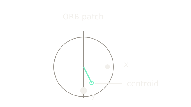
ORB uses intensity moments in a circular neighborhood. In a sparse synthetic patch, place intensity mass 1 at (1,0) and mass 2 at (0,1) relative to the keypoint. The centroid is (1/3,2/3); its direction is atan2(2,1)=63.435°. This scene uses image y downward and 80 drawing units per coordinate. Dot areas represent masses, and the mint hollow dot marks the centroid. ORB uses the moment direction, not the nearest bright pixel. A zero first-moment vector cannot define a stable angle. See the official ORB description.
Encode Binary Comparisons
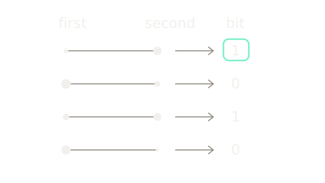
Read each pair from first to second; dot areas encode intensity, not sampling-window size. Tests (20,70), (90,30), (40,60) and (80,10) yield 1,0,1,0 under the convention I(first) < I(second). These four tests demonstrate the rule; a standard ORB descriptor with two-point tests has 256 bits. The actual pattern selects useful tests with high variance and low correlation. A single comparison close to equality can flip under noise.
Steer The Sampling Pattern
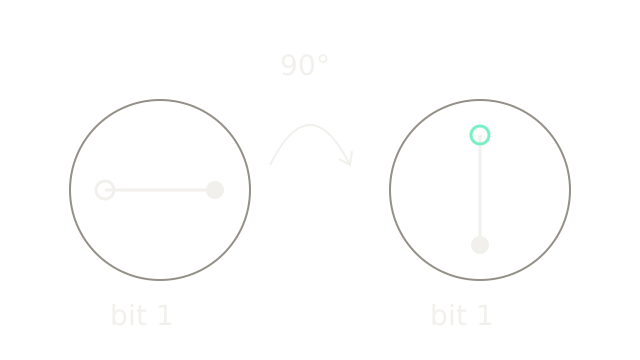
The hollow marker identifies the first sample and the solid marker the second; marker sizes now identify order rather than intensity. In image coordinates, a clockwise 90° rotation takes offsets (-1,0),(1,0) to (0,-1),(0,1). Steering the tests with the patch preserves which scene locations are compared, so the example remains bit 1 when the intensity ordering is unchanged. Sampling interpolation, orientation error and viewpoint changes can still alter the bits. ORB's orientation quantization further approximates this ideal rotation.
Where It Breaks
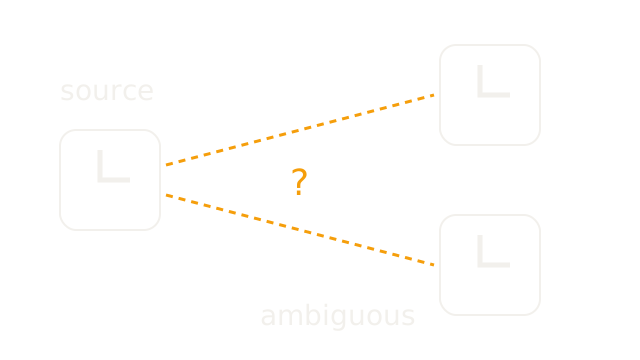
Two physically different L patches can look identical within the descriptor support. Both receive the same signature, leaving the dashed alternatives unresolved. Neither SIFT's normalization nor ORB's steering supplies missing context. Occlusion and large viewpoint changes can instead make a true match look different.
Compare SIFT descriptors with an appropriate vector metric such as L2 and standard two-point ORB descriptors with Hamming distance. ORB's WTA_K=3 or 4 requires OpenCV's Hamming2 norm. Appearance supplies candidates; feature matching and RANSAC tests ambiguity and geometric agreement. The official matcher reference specifies these norm choices.
The Quick Version
- Descriptors encode neighborhoods around detected image locations.
- Scale-aware support follows the apparent size of a feature.
- Relative orientations compensate for a shared patch rotation.
- SIFT pools gradient magnitudes into local direction bins.
- Sixteen eight-bin histograms form SIFT's 128-component descriptor.
- Normalization reduces sensitivity to uniform positive contrast changes.
- ORB estimates orientation toward the patch's intensity centroid.
- Ordered intensity comparisons produce ORB's binary tests.
- Steering rotates sampling offsets with the assigned orientation.
- Repeated local patterns remain ambiguous without additional evidence.