Image Histograms and Contrast Equalization

Count The Pixel Values

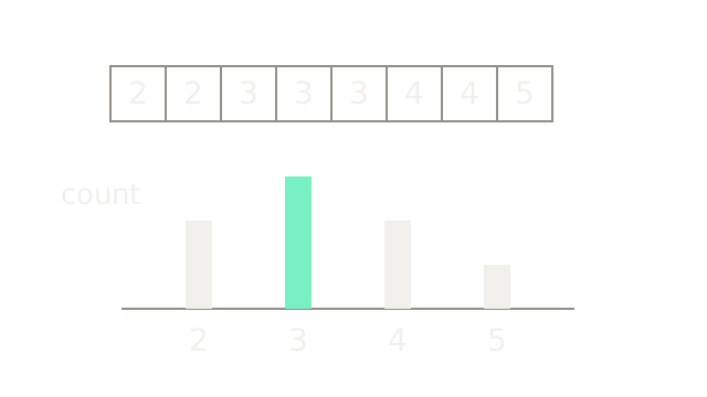
A histogram counts intensity values; histogram equalization uses their cumulative distribution to remap brightness. It can spread a narrow occupied range, but it cannot create distinctions absent from the input.

Our deliberately tiny 3-bit image has eight pixels: [2,2,3,3,3,4,4,5], with possible codes 0 through 7. The four bars count 2, 3, 2 and 1 pixels at levels 2, 3, 4 and 5. Each count adds 40 drawing units to the bar height; the counts sum to eight. Empty bins have zero height. Shuffling the pixels would leave this histogram unchanged: it contains no spatial arrangement.

Accumulate From Dark To Bright

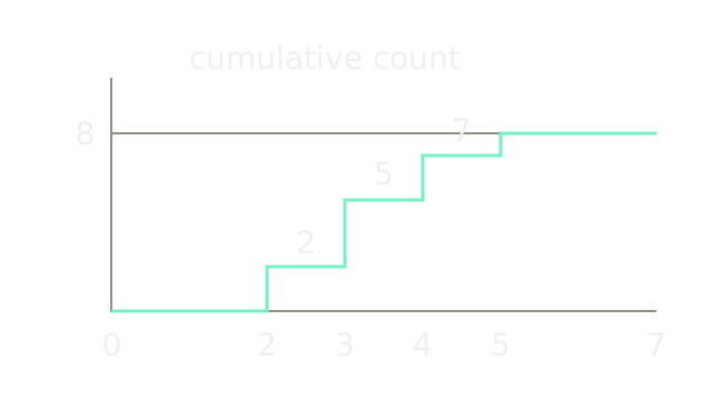
At level 2, two pixels are at or below that level. At level 3 there are 2+3 = 5; at 4 there are seven; at 5 there are eight. The staircase therefore reaches counts [2,5,7,8], remaining at eight through code 7. Divide by eight for the cumulative distribution: [0.25,0.625,0.875,1] at the occupied levels. Cumulative counts never decrease.

Build One Lookup

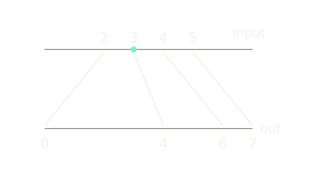
Both horizontal axes use the same level scale. Each sloping line joins an input level to its output. Use the minimum-nonzero-CDF subtraction shown in OpenCV's equalization walkthrough, with a nearest-integer rounding convention for this example:

$$T(r)=\operatorname{round}\left((L-1)\frac{C(r)-C_{\min}}{N-C_{\min}}\right).$$

Here L=8, N=8 and Cmin=2. Level 2 maps to round(7×0/6)=0; 3 maps to round(7×3/6)=4; 4 maps to round(7×5/6)=6; and 5 maps to round(7×6/6)=7. The 3.5 tie rounds upward here. Other definitions omit CDF-min subtraction or use different integer rounding; state the convention before comparing exact codes. A constant image needs a special case because this denominator becomes zero.

Spread Levels, Keep Groups

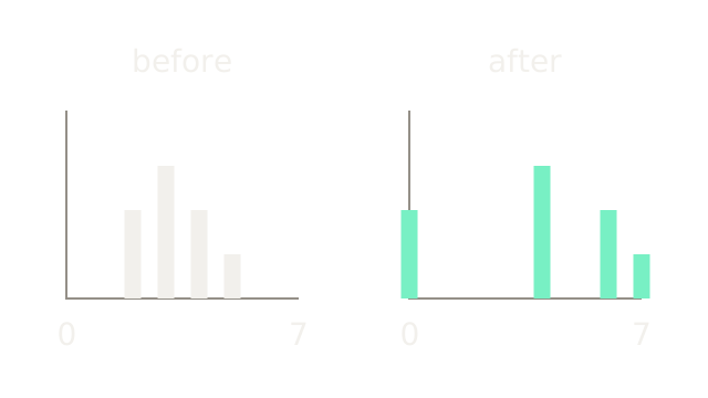
The output pixels are [0,0,4,4,4,6,6,7]. Both histograms share the same horizontal range, 0–7, and the same count scale. The level positions spread while the four group sizes remain 2, 3, 2 and 1. All three pixels originally at level 3 receive the same new value 4. A deterministic lookup cannot split that group to make perfectly uniform counts; rounding may also merge different input levels in other examples.

A Histogram Loses Position

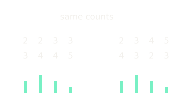
These are two different arrangements of our eight pixels. Both still contain two 2s, three 3s, two 4s and one 5. Their four count bars match exactly, although their boundaries and neighborhoods differ. A global histogram alone cannot tell where an object is or whether pixels form a connected shape. Applying the same global lookup to either image preserves that difference in arrangement; it does not rearrange pixels into histogram order.

Compare With Linear Stretching

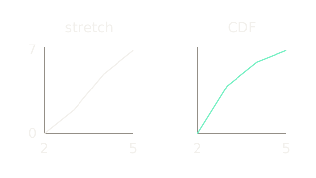
Linear stretching uses the occupied endpoints rather than frequency counts. For this fixture, round(7×(r−2)/(5−2)) maps [2,3,4,5] to [0,2,5,7]. Our equalization lookup maps them to [0,4,6,7]. Each plot has the same input and output scales; lines connect the four discrete lookup values. Both expand the occupied range to 0–7, but equalization allocates output intervals according to cumulative mass. They are different operations, even when both increase visible contrast.

Let The Neighborhood Matter

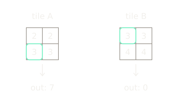
Use two new four-pixel tiles and the same 3-bit CDF-min rule. Tile A has [2,2,3,3], so level 3 reaches its maximum cumulative count and maps to 7. Tile B has [3,3,4,4], so level 3 is its first occupied bin and maps to 0. The outlined input values are both 3. These toy local lookups illustrate context; they are not exact OpenCV CLAHE outputs, whose lookup construction does not subtract CDF-min. A local mapping uses neighborhood context, whereas one global lookup must map every 3 identically. Independently applying such tile mappings would cause abrupt transitions at their boundaries.

Blend Across Tile Boundaries

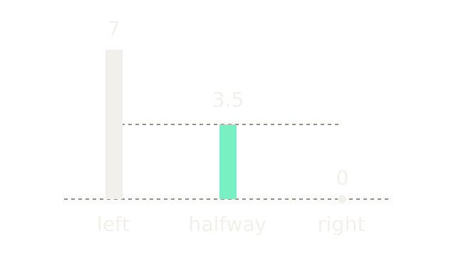
For that same input level, suppose neighboring lookup predictions are 7 and 0. A location halfway between their centers gives equal spatial weights, producing 0.5×7 + 0.5×0 = 3.5 before integer conversion. A quarter of the way across would instead give 5.25. This one-dimensional slice illustrates interpolation of lookup outputs for the current input, not averaging two neighboring source pixels. Two-dimensional implementations interpolate neighboring tile mappings to reduce visible seams.

Limit Histogram Peaks

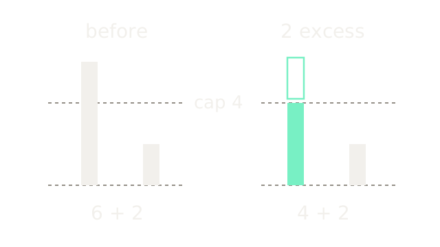
This separate eight-pixel toy histogram has nonzero bin counts 6 and 2. Clipping the first bin at a count of 4 leaves counts 4 and 2 plus two saved excess counts. The detached outlined segment is that excess; it is subsequently redistributed across histogram bins before building the cumulative mapping. Total mass remains eight. The image shows the clipping stage, not the final redistributed histogram or a particular library's integer redistribution algorithm.

OpenCV's CLAHE reference combines local equalization, histogram contrast limiting and interpolation. Its implementation scales the configured clip-limit parameter by tile area divided by bin count; the illustrative raw count cap of 4 here is not a recommendation for that API parameter. Histogram clipping limits how aggressively mappings amplify differences. It does not clamp bright image pixels like sensor saturation does.

Where It Breaks

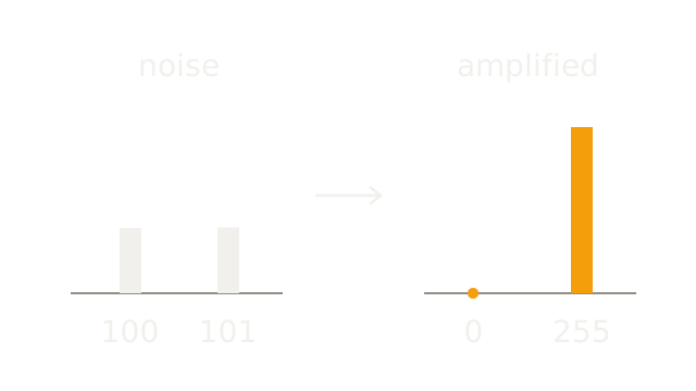
Switch to an 8-bit patch containing equally many 100s and 101s, differing only through noise. The same CDF-min rule maps them to 0 and 255. The vertical scale is identical before and after; a barely visible difference becomes maximal contrast. Equalization responds to the distribution, without knowing whether variation is useful signal.

Global contrast changes may also harm a region that already looks appropriate. CLAHE computes local mappings and clips histogram peaks to limit contrast amplification; it still does not recover lost detail. For color images, independently equalizing RGB channels can change color balance. Choose a suitable brightness-related channel and inspect the result rather than treating equalization as universally beneficial.

The Quick Version

• Histograms count values and discard their spatial arrangement.
• Cumulative counts measure how many pixels lie below each level.
• Equalization converts cumulative counts into a monotone intensity lookup.
• Equal input values remain equal; discrete histograms need not flatten.
• Pixel rearrangements can share identical histograms.
• Linear stretching uses endpoints; equalization uses cumulative counts.
• Local mappings adapt to neighborhood distributions.
• Interpolating tile mappings reduces abrupt spatial transitions.
• Contrast limiting clips histogram counts and redistributes excess mass.
• Noise can become stronger when a narrow range is stretched.