Early CNN Architectures

From handwritten digits in LeNet-5 to GPU-scaled AlexNet and uniform 3x3 stacks in VGG, each milestone proved deeper layers extract richer features.

Structural comparison of early CNN milestones: LeNet-5, AlexNet, and VGG-16 with 3x3 filter factorization.

Why Does This Exist?

Prior to 2012, computer vision systems relied on hand-engineered visual descriptors such as SIFT (Scale-Invariant Feature Transform) and HOG (Histogram of Oriented Gradients), paired with linear Support Vector Machines. These pipelines were brittle: if illumination, pose, or background clutter shifted, manually tuned feature extractors discarded the essential semantic signal.

Early convolutional neural networks proved that visual hierarchies could instead be learned directly from raw pixels using gradient descent. However, building deeper architectures hit immediate roadblocks: vanishing gradients with saturating activations, hardware memory limits on consumer GPUs, and an explosion of model parameters in dense classification heads.

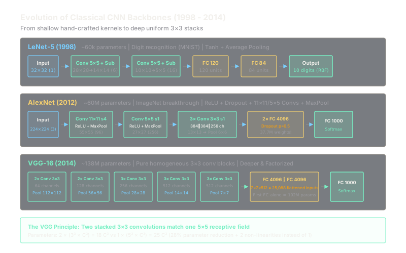
Understanding LeNet-5 (1998), AlexNet (2012), and VGGNet (2014) is essential because each network solved a foundational architectural dilemma:

LeNet-5 established the canonical pattern of alternating convolutions, spatial subsampling, and fully connected layers.
AlexNet demonstrated how ReLU non-linearities, dropout, data augmentation, and dual-GPU parallel execution could train an 8-layer deep network on 1.2 million ImageNet images.
VGGNet proved that replacing large filters ( $11 \times 11$ and $5 \times 5$ ) with homogeneous stacks of small $3 \times 3$ convolutions reduces parameters while boosting model non-linearity.

Think of It Like This

Telescopes, wide lenses, and micro-lens arrays

Imagine learning to photograph bird species in the wild. LeNet-5 is like a simple handheld spyglass: it can cleanly distinguish black ink digits printed on bank checks, but its tiny lens cannot resolve the chaotic feathers and dense branches of real-world scenes.

AlexNet is a heavy safari camera with multiple oversized interchangeable lenses: an ultra-wide $11 \times 11$ lens to quickly sweep the horizon, followed by a $5 \times 5$ lens for medium objects, and smaller lenses for fine plumage. It captures stunning detail across 1,000 animal categories, but swapping between awkwardly sized lenses is heavy, clunky, and burns massive power.

VGGNet standardizes the entire camera setup using uniform micro-lenses. Instead of carrying huge, specialized lenses, it stacks modular, identical $3 \times 3$ optical filters in series. Two consecutive small filters give the exact same field of view as one giant lens, but they weigh 28% less and allow the photographer to insert multiple intermediate color filters in between.

How It Actually Works

The Structural Evolution

1LeNet-5 (1998):   Input (32×32×1)  ➔ Conv 5×5 (6)  ➔ AvgPool ➔ Conv 5×5 (16) ➔ AvgPool ➔ FC 120 ➔ FC 84 ➔ Out 102AlexNet (2012):   Input (224×224×3) ➔ Conv 11×11 (96, s=4) ➔ MaxPool ➔ Conv 5×5 (256) ➔ MaxPool ➔ 3× Conv 3×3 ➔ 2× FC 4096 ➔ Out 10003VGG-16 (2014):    Input (224×224×3) ➔ [2× Conv 3×3 (64)] ➔ [2× Conv 3×3 (128)] ➔ [3× Conv 3×3 (256)] ➔ [3× Conv 3×3 (512)] ➔ [3× Conv 3×3 (512)] ➔ 2× FC 4096 ➔ Out 1000

LeNet-5 (Yann LeCun et al.): Designed for digit recognition on the MNIST benchmark. Used sigmoid and hyperbolic tangent ( $\tanh$ ) activations. Crucially, subsampling was average pooling with learnable coefficients and biases:

a_j = f\left(\beta_j \sum_{n \times n} a_i + b_j\right)

Total parameter count was modest: $\sim 60\text{,}000$ weights.

AlexNet (Alex Krizhevsky, Ilya Sutskever, Geoffrey Hinton): Won ImageNet 2012 by slashing the top-5 error rate from 26.2% to 15.3%. Key innovations included:
- ReLU non-linearity: $f(x) = \max(0, x)$ eliminated the vanishing gradient problem in positive regimes, accelerating convergence by $6\times$ compared to $\tanh$ .
- Overlapping Max Pooling: Kernel size $3 \times 3$ with stride $S=2$ , reducing spatial dimensions while mitigating blurring.
- Dropout ( $p=0.5$ ): Applied to the two 4,096-neuron fully connected layers to prevent severe co-adaptation.
- Heavy Parameter Allocation: 60 million parameters, where the transition from convolutional maps to FC 4096 alone accounted for nearly 38 million parameters ( $6 \times 6 \times 256 \times 4096 \approx 37.7 \times 10^6$ ).
VGGNet (Simonyan and Zisserman): Investigated network depth using uniform $3 \times 3$ filters with stride $S=1$ and padding $P=1$ , alongside $2 \times 2$ max pooling ( $S=2$ ).

Mathematical Factorization: Stacking $3 \times 3$ Convolutions

Consider two stacked convolutional layers, each with kernel size $K=3$ and stride $S=1$ .

The receptive field $R_l$ of layer $l$ is calculated recursively:

R_l = R_{l-1} + (K_l - 1) \cdot \prod_{i=1}^{l-1} S_i

For layer 1: $R_1 = 1 + (3 - 1) \cdot 1 = 3$ . For layer 2: $R_2 = 3 + (3 - 1) \cdot 1 = 5$ .

Thus, a stack of two $3 \times 3$ layers covers an effective $5 \times 5$ spatial receptive field. Similarly, a stack of three $3 \times 3$ layers covers an effective $7 \times 7$ field:

R_3 = 5 + (3 - 1) \cdot 1 = 7

Parameter and FLOP Efficiency

Assume both the input and output have $C$ feature channels:

A single $5 \times 5$ convolution requires:

\text{Params}(5 \times 5) = 5 \times 5 \times C \times C = 25 C^2

Two stacked $3 \times 3$ convolutions require:

\text{Params}(2 \times 3 \times 3) = 2 \times (3 \times 3 \times C \times C) = 18 C^2

The parameter ratio is:

\frac{18 C^2}{25 C^2} = 0.72 \quad (28\% \text{ reduction in parameters})

Furthermore, the stacked architecture applies two non-linear activation functions (e.g., ReLU) rather than one, increasing functional expressiveness.

Worked Example

Let us compute the total parameter count and activation tensor dimensions for a VGG block taking an input tensor of shape $X \in \mathbb{R}^{64 \times 112 \times 112}$ and transforming it into 128 channels through two $3 \times 3$ convolutions (with bias), followed by $2 \times 2$ max pooling ( $S=2$ ):

Layer 1: Conv2d(64, 128, kernel_size=3, padding=1):
- Output spatial dimension: $\lfloor (112 - 3 + 2)/1 \rfloor + 1 = 112$ .
- Output tensor shape: $(128, 112, 112)$ .
- Weights: $128 \times 64 \times 3 \times 3 = 73\text{,}728$ .
- Biases: $128$ .
- Layer 1 parameters: $73\text{,}728 + 128 = 73\text{,}856$ .
Layer 2: Conv2d(128, 128, kernel_size=3, padding=1):
- Output spatial dimension: $112$ .
- Output tensor shape: $(128, 112, 112)$ .
- Weights: $128 \times 128 \times 3 \times 3 = 147\text{,}456$ .
- Biases: $128$ .
- Layer 2 parameters: $147\text{,}456 + 128 = 147\text{,}584$ .
Layer 3: MaxPool2d(kernel_size=2, stride=2):
- Output spatial dimension: $\lfloor (112 - 2)/2 \rfloor + 1 = 56$ .
- Output tensor shape: $(128, 56, 56)$ .
- Parameters: $0$ .

Total parameters in this VGG stage: $73\text{,}856 + 147\text{,}584 = 221\text{,}440$ weights.

Code

1import torch2import torch.nn as nn3
4class VGGBlock(nn.Module):5    """A standard two-layer VGG convolutional stage with 3x3 filters."""6    def __init__(self, in_channels: int, out_channels: int) -> None:7        super().__init__()8        self.block = nn.Sequential(9            nn.Conv2d(in_channels, out_channels, kernel_size=3, padding=1),10            nn.ReLU(inplace=True),11            nn.Conv2d(out_channels, out_channels, kernel_size=3, padding=1),12            nn.ReLU(inplace=True),13            nn.MaxPool2d(kernel_size=2, stride=2)14        )15
16    def forward(self, x: torch.Tensor) -> torch.Tensor:17        return self.block(x)18
19# Input tensor simulating intermediate feature map: Batch=2, C=64, H=112, W=11220x = torch.randn(2, 64, 112, 112)21vgg_stage = VGGBlock(in_channels=64, out_channels=128)22
23out = vgg_stage(x)24print(out.shape)25# -> torch.Size([2, 128, 56, 56])26
27# Parameter count calculation28total_params = sum(p.numel() for p in vgg_stage.parameters())29print(total_params)30# -> 221440

Watch Out For

Massive parameter memory traps in dense classification heads

In AlexNet and VGG-16, the fully connected classifier heads account for over 70% to 80% of total network parameters. In VGG-16, the final pooling layer outputs a feature map of shape $512 \times 7 \times 7 = 25\text{,}088$ . Projecting this into the first FC 4096 layer requires $25\text{,}088 \times 4096 + 4096 \approx 102.7 \times 10^6$ parameters.

This creates severe memory bottlenecks during distributed training and high risk of overfitting on smaller datasets. Modern architectures solve this by replacing oversized dense heads with Global Average Pooling (GAP), which averages each $H \times W$ feature map into a single scalar ( $1 \times 1 \times C$ ), followed by a single lightweight linear projection layer.

The Quick Version

LeNet-5 established the foundational blueprint of alternating convolutions, downsampling, and dense classifiers.
AlexNet catalyzed deep learning by pairing GPU training with ReLU activations, dropout regularization, and large-scale data.
VGGNet proved that stacking small $3 \times 3$ convolutions provides the exact same receptive field as larger kernels with 28% fewer parameters and higher non-linearity.
The dense classification heads of early architectures were notoriously parameter-heavy, leading modern networks to adopt Global Average Pooling.
Two $3 \times 3$ convolutions yield an effective $5 \times 5$ receptive field; three $3 \times 3$ convolutions cover $7 \times 7$ .