The Inception Family

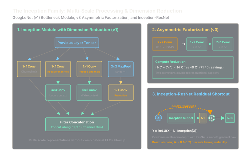
Instead of choosing one filter size, Inception runs 1x1, 3x3, and 5x5 convolutions in parallel at the same layer, using 1x1 bottlenecks to keep compute low.

Inception module with multi-scale parallel branches, 1x1 dimensionality reduction, asymmetric factorization, and residual connections.

Why Does This Exist?

In real-world visual scenes, salient objects appear at radically different scales. An image might contain a massive face occupying 80% of the camera view, or a flock of tiny birds taking up only 10 pixels each. Choosing a single fixed convolutional kernel size creates an architectural dilemma:

Small kernels ( $3 \times 3$ ) capture fine edge details but fail to integrate global context without dozens of stacked layers.
Large kernels ( $5 \times 5$ or $7 \times 7$ ) capture broad spatial relationships but are computationally expensive, squaring FLOP requirements and washing out fine local boundaries.

Before the Inception architecture (GoogLeNet, Szegedy et al., 2014), networks simply committed to a uniform kernel size per layer. Making networks wider or deeper quickly caused computational explosion: VGG-16 required 138 million parameters and $\sim 15.5$ billion multiply-accumulate operations per forward pass.

The Inception architecture solved this by operating across multiple spatial scales simultaneously within the same layer block. By introducing $1 \times 1$ "bottleneck" convolutions before expensive spatial filters, GoogLeNet built a 22-layer network with just 6.8 million parameters—less than 5% of VGG's parameter footprint—while outperforming it on ImageNet.

Think of It Like This

An investigative news desk with specialized reporters

Imagine a newsroom covering a major breaking event. A traditional news bureau assigns one reporter with one specific reporting style per edition: yesterday was an aerial helicopter survey, today is an on-the-ground interview, tomorrow is a headline desk summary.

An Inception module is a multi-specialist investigative desk that deploys four reporters simultaneously for every single story:

One reporter runs a quick $1 \times 1$ fact-check on background data.
A second reporter zooms in on local details with a $3 \times 3$ street lens.
A third reporter views the broad panoramic context with a $5 \times 5$ regional lens.
A fourth reporter monitors the most active trends using a $3 \times 3$ max-pooling filter.

Crucially, before sending reporters on expensive $3 \times 3$ and $5 \times 5$ fieldwork, an editor uses a $1 \times 1$ filter to summarize hundreds of rambling news wires down to just 32 key talking points. When all four reporters return, their articles are bound side-by-side into a single comprehensive briefing.

How It Actually Works

The Multi-Scale Inception Block with Bottlenecks

The naive Inception module routes the input tensor $X \in \mathbb{R}^{C_{\text{in}} \times H \times W}$ into four parallel paths:

$1 \times 1$ convolution
$3 \times 3$ convolution
$5 \times 5$ convolution
$3 \times 3$ max pooling

If $C_{\text{in}} = 256$ and each branch produces 128 channels, convolving 256 channels directly with $5 \times 5$ filters explodes compute: $256 \times 128 \times 5 \times 5 \times H \times W \approx 819\text{,}200 \times H \times W$ FLOPs.

The solution is the $1 \times 1$ bottleneck convolution. A $1 \times 1$ convolution computes a linear combination across input channels at each pixel:

Y_{\text{red}}[c, i, j] = \sum_{k=0}^{C_{\text{in}}-1} X[k, i, j] \cdot W_{1\times 1}[c, k]

By setting the intermediate channel count $C_{\text{mid}} \ll C_{\text{in}}$ (for instance, reducing from 256 to 32), the subsequent $5 \times 5$ convolution only computes against 32 channels. Finally, all four branch outputs are concatenated along the channel dimension:

Y_{\text{concat}} = \left[ Y_{1\times 1} \,\|\, Y_{3\times 3} \,\|\, Y_{5\times 5} \,\|\, Y_{\text{pool\_proj}} \right] \in \mathbb{R}^{(C_1 + C_2 + C_3 + C_4) \times H \times W}

Architectural Evolution Across Generations

The Inception family evolved across four major iterations:

Inception v1 (GoogLeNet, 2014): Introduced the 4-branch module with $1 \times 1$ bottlenecks and auxiliary classification heads to inject training gradients directly into intermediate layers.
Inception v2 / Batch Normalization (Ioffe & Szegedy, 2015): Replaced $5 \times 5$ convolutions with two stacked $3 \times 3$ convolutions ( $25 C^2 \to 18 C^2$ parameters) and introduced Batch Normalization.
Inception v3 (Szegedy et al., 2016): Introduced asymmetric convolution factorization:
- Factoring an $n \times n$ filter into an $1 \times n$ followed by an $n \times 1$ convolution:
$\text{FLOPs}(1 \times n + n \times 1) = (n + n) \cdot C^2 = 2n \cdot C^2 \quad \text{vs.} \quad n^2 \cdot C^2$ For $n=7$ $n = 7$ , $1 \times 7 + 7 \times 1$ $1 \times 7 + 7 \times 1$ uses 14 operations instead of 49—a 71.4% computational reduction.
- Introduced label smoothing and RMSProp optimization.
Inception-ResNet-v1 & v2 (Szegedy et al., 2017): Blended Inception multi-scale blocks with ResNet residual identity shortcuts: $Y = \text{ReLU}\left(X + \lambda \cdot \mathcal{F}_{\text{Inception}}(X)\right)$ where $\lambda \in [0.1, 0.2]$ is a residual scaling factor preventing the network from dying when channel counts exceed 1,000.

Worked Example

Let us compute the exact number of multiply-accumulate (MAC) operations for an input tensor $X \in \mathbb{R}^{256 \times 28 \times 28}$ processed by a $5 \times 5$ branch producing 128 output channels:

Naive Branch (No Bottleneck):
- Direct Conv2d(256, 128, kernel=5, padding=2):
$\text{MACs}_{\text{naive}} = H \times W \times C_{\text{in}} \times C_{\text{out}} \times K^2 = 28 \times 28 \times 256 \times 128 \times 25 = 642\text{,}252\text{,}800 \text{ MACs} \approx 642.3\text{ M}$
Inception Bottleneck Branch ( $1 \times 1$ reduction to 32 channels, then $5 \times 5$ ):
- Step A: Conv2d(256, 32, kernel=1, padding=0):
$\text{MACs}_{1\times 1} = 28 \times 28 \times 256 \times 32 \times 1 = 6\text{,}422\text{,}528 \text{ MACs} \approx 6.42\text{ M}$
- Step B: Conv2d(32, 128, kernel=5, padding=2):
$\text{MACs}_{5\times 5} = 28 \times 28 \times 32 \times 128 \times 25 = 80\text{,}281\text{,}600 \text{ MACs} \approx 80.28\text{ M}$
- Total MACs with bottleneck:
$6.42\text{ M} + 80.28\text{ M} = 86.70\text{ M MACs}$

The bottleneck reduces compute by:

\frac{86.70\text{ M}}{642.25\text{ M}} \approx 13.5\% \text{ of the original compute} \quad (86.5\% \text{ reduction!})

Code

1import torch2import torch.nn as nn3
4class InceptionBlock(nn.Module):5    """Classic Inception v1 (GoogLeNet) block with 1x1 bottleneck projections."""6    def __init__(7        self,8        in_channels: int,9        n1x1: int,10        n3x3_reduce: int,11        n3x3: int,12        n5x5_reduce: int,13        n5x5: int,14        pool_proj: int15    ) -> None:16        super().__init__()17        # Branch 1: 1x1 conv18        self.branch1 = nn.Sequential(19            nn.Conv2d(in_channels, n1x1, kernel_size=1),20            nn.ReLU(inplace=True)21        )22        # Branch 2: 1x1 conv -> 3x3 conv23        self.branch2 = nn.Sequential(24            nn.Conv2d(in_channels, n3x3_reduce, kernel_size=1),25            nn.ReLU(inplace=True),26            nn.Conv2d(n3x3_reduce, n3x3, kernel_size=3, padding=1),27            nn.ReLU(inplace=True)28        )29        # Branch 3: 1x1 conv -> 5x5 conv (using same padding=2)30        self.branch3 = nn.Sequential(31            nn.Conv2d(in_channels, n5x5_reduce, kernel_size=1),32            nn.ReLU(inplace=True),33            nn.Conv2d(n5x5_reduce, n5x5, kernel_size=5, padding=2),34            nn.ReLU(inplace=True)35        )36        # Branch 4: 3x3 max pool -> 1x1 conv37        self.branch4 = nn.Sequential(38            nn.MaxPool2d(kernel_size=3, stride=1, padding=1),39            nn.Conv2d(in_channels, pool_proj, kernel_size=1),40            nn.ReLU(inplace=True)41        )42
43    def forward(self, x: torch.Tensor) -> torch.Tensor:44        out1 = self.branch1(x)45        out2 = self.branch2(x)46        out3 = self.branch3(x)47        out4 = self.branch4(x)48        return torch.cat([out1, out2, out3, out4], dim=1)49
50# Input tensor: Batch=2, C=256, H=28, W=2851x = torch.randn(2, 256, 28, 28)52block = InceptionBlock(53    in_channels=256,54    n1x1=64,55    n3x3_reduce=64,56    n3x3=128,57    n5x5_reduce=32,58    n5x5=32,59    pool_proj=3260)61
62out = block(x)63print(out.shape)64# -> torch.Size([2, 256, 28, 28])

Watch Out For

Representational bottlenecks and unstable wide Inception-ResNets

Two common pitfalls occur when building Inception networks:

Representational Bottlenecks: Aggressively reducing channel dimensions too early in the network discards critical spatial signals. The information theoretic principle stated in Inception v3 dictates that representation dimension should gently expand from inputs to classification outputs before pooling.
Residual Explosion in Inception-ResNet: When intermediate Inception-ResNet channel counts exceed 1,000, unscaled residual addition causes activations to explode in value before ReLU, resulting in zero gradients and dead networks early in training. Always apply residual scaling ( $\lambda \in [0.1, 0.2]$ ) to multiply the Inception branch output before the residual sum.

The Quick Version

The Inception architecture runs parallel convolutions ( $1 \times 1, 3 \times 3, 5 \times 5$ ) and pooling at the same depth to process multi-scale visual features.
$1 \times 1$ convolutions act as learned channel bottlenecks, cutting arithmetic by over 80% prior to larger spatial filters.
Inception v2 replaced $5 \times 5$ filters with two stacked $3 \times 3$ filters; Inception v3 factored $n \times n$ into asymmetric $1 \times n$ and $n \times 1$ pairs.
Inception-ResNet combines multi-scale Inception diversity with residual identity shortcuts for fast convergence.
Scale the residual branch by $\lambda \approx 0.1$ when building deep Inception-ResNet networks to avoid activation divergence.