Encoder-Decoder Segmentation Architectures

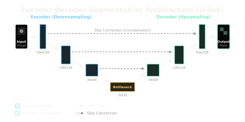
By pairing a downsampling encoder to capture deep semantic context with an upsampling decoder to recover spatial details, models like U-Net can classify every pixel in an image.

An encoder compresses the image to understand 'what' is present, while a decoder expands it back up using skip connections to remember 'where' it was, yielding a dense pixel-wise map.

Why Does This Exist?

Traditional convolutional neural networks (CNNs) are exceptional at classifying entire images. Through progressive pooling and striding, they compress a large spatial grid into a tiny feature vector that summarizes what is in the image, discarding exactly where it was. However, for tasks like medical imaging or autonomous driving, we need dense predictions: we must classify every single pixel. We need the deep contextual understanding of a classifier, combined with the precise localization of the original resolution. Encoder-decoder segmentation architectures solve this by running the classification process in reverse, expanding the deep features back to full size.

Think of It Like This

A detective and a forensic artist

Imagine a detective analyzing a crime scene photo. To understand the whole story (the "context"), the detective steps back, squinting to see the big picture (the encoder). They figure out that there's a car, a tree, and a person. But to draw a precise map of the scene, a forensic artist needs exact details (the decoder). The artist takes the detective's high-level summary and combines it with earlier, high-resolution notes taken before stepping back (the skip connections). Together, they produce a high-fidelity, labeled map of the entire scene.

How It Actually Works

The architecture consists of three primary mechanisms working in tandem:

1. The Encoder (Contracting Path)

The encoder looks exactly like a standard classification network (e.g., ResNet or VGG). It applies a series of convolutional filters followed by pooling layers (or strided convolutions). With each block, the spatial dimensions (height and width) shrink, but the number of channels (feature depth) increases. This captures high-level semantic information (the "what") and increases the receptive field, allowing the network to understand large objects and context.

2. The Decoder (Expanding Path)

To recover the original resolution, the decoder takes the tiny, deep feature map and progressively scales it up. This is typically done using transposed convolutions or bilinear upsampling followed by standard convolutions. While upsampling increases the spatial resolution, it inherently guesses missing details because pooling in the encoder destroyed exact positional information.

3. Skip Connections

This is the breakthrough introduced by U-Net and Fully Convolutional Networks (FCNs). To recover the fine-grained spatial details lost during pooling, the network uses skip connections. Before a feature map in the encoder is pooled and downsampled, a copy is routed directly across to the corresponding stage in the decoder. The decoder concatenates this high-resolution feature map with its upsampled features. This allows the decoder to seamlessly merge deep, contextual semantics with shallow, precise localization.

Code

1import torch2import torch.nn as nn3
4class SimpleUNet(nn.Module):5    def __init__(self):6        super().__init__()7        # Encoder: 1 channel -> 64 channels (downsampled)8        self.enc_conv = nn.Conv2d(1, 64, kernel_size=3, padding=1)9        self.pool = nn.MaxPool2d(2)10        11        # Bottleneck: 64 -> 128 channels12        self.bottleneck = nn.Conv2d(64, 128, kernel_size=3, padding=1)13        14        # Decoder: Upsample 128 -> 64 channels15        self.up = nn.ConvTranspose2d(128, 64, kernel_size=2, stride=2)16        # Merge skip connection (64 + 64 = 128 channels) -> 64 channels17        self.dec_conv = nn.Conv2d(128, 64, kernel_size=3, padding=1)18        19        # Output: 64 -> 2 classes (e.g., background vs object)20        self.out = nn.Conv2d(64, 2, kernel_size=1)21
22    def forward(self, x):23        # 1. Encoder step24        skip = torch.relu(self.enc_conv(x))25        down = self.pool(skip)26        27        # 2. Bottleneck28        deep = torch.relu(self.bottleneck(down))29        30        # 3. Decoder with skip connection31        up = self.up(deep)32        # Concatenate skip connection along channel dimension33        merged = torch.cat([up, skip], dim=1)34        35        out_features = torch.relu(self.dec_conv(merged))36        return self.out(out_features) # -> [Batch, 2, H, W]

Watch Out For

Spatial mismatch in skip connections

If your input image dimensions are not neatly divisible by $2^N$ (where $N$ is the number of pooling layers), the upsampled decoder features will have a different spatial size than the encoder's skip connections. Attempting to concatenate them will throw a tensor shape mismatch error. Always pad your inputs or use crop-and-concat operations if dimensions misalign.

The Quick Version

Classification networks lose spatial detail; segmentation requires dense, pixel-by-pixel output.
The encoder downsamples the image to capture broad semantic context ("what is it").
The decoder upsamples the deep features back to the original resolution.
Skip connections copy high-resolution features directly from the encoder to the decoder, restoring the lost spatial precision ("where is it").
U-Net is the quintessential example, shaping the architecture like a 'U' due to its symmetric paths and horizontal skip connections.