Graph Neural Networks for Vision

Objects in a scene relate to each other, and keypoints sit on irregular grids. Graph networks turn regions or points into nodes and let messages pass along the edges before anyone decides.

One message-passing round updates each region from its graph neighbors, so the middle node blends both sides

Why Does This Exist?

Convolutions assume a fixed grid, but much of vision is not grid-shaped. A human skeleton is seventeen joints wired by bones; a scene is a handful of regions with "next to" and "holding" between them; a point cloud is coordinates with no order at all. Forcing these into rectangles either destroys the relations or pads them into wasteful regularity.

Graph neural networks take the relations as the input format. Nodes carry features (a region's appearance, a joint's position), edges carry the structure (adjacency, bones, proximity), and learning happens by passing messages along the edges. This page covers message passing for vision graphs. The symmetry view is geometric deep learning; the region input usually comes from object detection.

The one idea you need first. Message passing updates every node from its neighbors in two moves: aggregate (pool the neighbors' features, by mean, sum, or attention) and update (combine the pooled message with the node's own feature through a small network). Reordering the nodes changes nothing, because pooling ignores order — that permutation equivariance is the whole reason graphs generalize across scenes with different object counts.

Think of It Like This

Neighborhood gossip, one round

Every house on the street starts the morning with its own news. At noon each household steps out, listens to its immediate neighbors, and revises its story: your news plus the average of next door. Nobody hears the far end of the street yet — that takes more rounds.

A GNN layer is that noon revision. Aggregation is listening; the update is revising. After one round each node knows its neighborhood, after two it knows its neighbors' neighborhoods, and the street's far end stays rumor until the rounds reach it. Depth in a GNN is counted in gossip rounds, not in pixels.

The analogy stops at trust: neighbors in a GNN are weighted by learned attention, not by who shouts loudest, and too many rounds melt every story into the same average.

How It Actually Works

Build the graph first: regions become nodes with appearance features, and edges connect spatial neighbors (or bones for skeletons, or k-nearest neighbors for point clouds). One message-passing layer computes, for each node, the mean of its neighbors' features (including itself), then applies a linear map plus nonlinearity. Stacking layers widens each node's receptive field by one hop per layer. A final readout pools all nodes for image-level decisions or keeps per-node outputs for region labeling.

Choices that matter: mean versus attention aggregation (attention helps when some neighbors are irrelevant), residual connections between rounds (they slow the slide into uniformity), and graph construction itself, which is often more decisive than the layer math.

Worked example

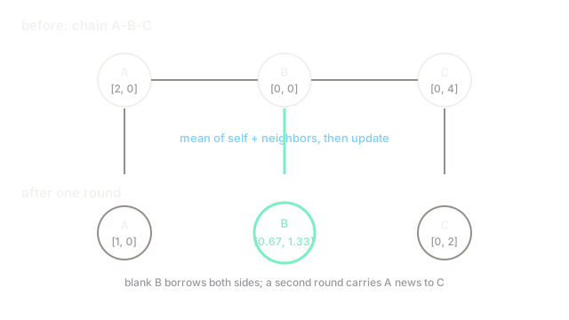
Three regions in a chain A–B–C with 2-D appearance features:

$A = [2, 0], \quad B = [0, 0], \quad C = [0, 4]$

One mean-aggregation round (each node pools itself plus its neighbors):

$A$ pools $\{A, B\}$ : $[(2 + 0)/2,\ (0 + 0)/2] = [1, 0]$ .
$B$ pools $\{A, B, C\}$ : $[(2 + 0 + 0)/3,\ (0 + 0 + 4)/3] = [0.67,\ 1.33]$ .
$C$ pools $\{B, C\}$ : $[(0 + 0)/2,\ (0 + 4)/2] = [0,\ 2]$ .

The middle node $B$ now carries both sides' evidence $[0.67, 1.33]$ : blank on its own, informative after listening. A second round would carry $A$ 's news to $C$ through $B$ .

Code

The point of this snippet is the round: neighbor lists plus mean pooling reproduce the worked example exactly.

1features = {"A": [2.0, 0.0], "B": [0.0, 0.0], "C": [0.0, 4.0]}2neighbors = {"A": ["A", "B"], "B": ["A", "B", "C"], "C": ["B", "C"]}3
4
5def message_pass(features: dict, neighbors: dict) -> dict:6    out = {}7    for node, group in neighbors.items():  # pool self plus neighbors8        pooled = [sum(features[n][d] for n in group) / len(group) for d in range(2)]9        out[node] = [round(v, 2) for v in pooled]10    return out11
12
13print(message_pass(features, neighbors))  # -> {'A': [1.0, 0.0], 'B': [0.67, 1.33], 'C': [0.0, 2.0]}

Watch Out For

Oversmoothing melts every node into the average

Each round mixes neighbors closer together. After many rounds on a connected graph, all node features converge toward one shared vector and region distinctions vanish — accuracy rises for a few layers, then slides for every added one.

Treat depth as hops needed, not layers wanted: two to four rounds cover most vision graphs. Add residuals between rounds and watch per-node feature variance during training; when it collapses, the network is gossiping, not reasoning.

Dense graphs explode the neighbor lists

Connecting every region to every other turns one round into quadratic work and drowns each node in irrelevant messages. Full attention over hundreds of superpixels is slow and usually worse than sparse structure.

Sparsify deliberately: k-nearest spatial neighbors, skeleton bones, or learned top-k edges. The graph construction is a modeling decision with larger effects than the aggregation formula most teams tune first.

The Quick Version

GNNs represent scenes as nodes (regions, joints, points) with edges for their relations.
One round aggregates neighbor features and updates each node; order never matters.
The worked fixture turns blank node $B$ into $[0.67, 1.33]$ by pooling both neighbors.
Depth is gossip rounds: too many rounds oversmooth every node into the same average.
Sparse, meaningful edges beat dense ones for both speed and accuracy.