Graph Cut Segmentation

Turn the image into a plumbing network where cutting cheap pipes separates foreground from background at the lowest total cost. The minimum cut is the segmentation.

The cheapest source-to-sink cut equals the lowest-energy labeling, balancing pixel evidence against neighbour agreement.

Why Does This Exist?

Per-pixel rules like thresholding label each pixel in isolation, so one noisy pixel flips alone and borders come out ragged. Real segmentations should be smooth: neighbours usually share a label, and disagreeing with a similar neighbour ought to cost something. Graph cut makes that tradeoff exact by writing segmentation as an energy and finding its global minimum, something greedy methods like snakes cannot promise for binary labels.

This page covers the graph construction, the two energy terms, and the minimum-cut answer. The interactive descendant that removes the need for per-pixel seeds is GrabCut; the boundary-evolution alternative is active contours.

Think of It Like This

Cutting a power grid at lowest cost

Two power stations feed one grid and you must separate their territories by cutting wires, paying each wire's capacity as the cutting cost. Cut wires nobody needs and the bill stays small; cut a trunk line and it spikes. The cheapest set of cuts that fully separates the stations is the answer, and no cheaper separation exists.

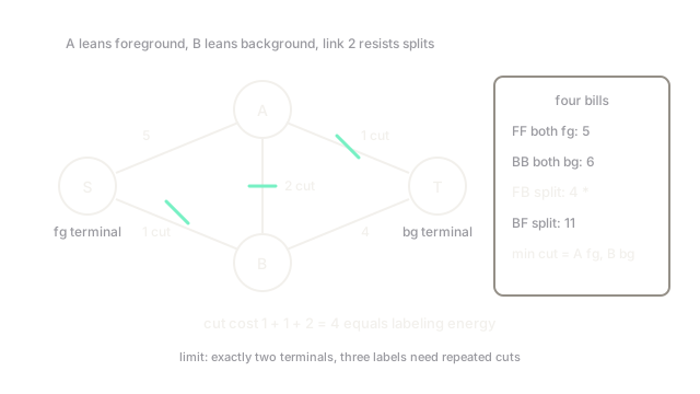
It stops holding past two stations. The min-cut machinery separates exactly two terminals, foreground versus background, so three or more labels need repeated cuts or different machinery entirely.

How It Actually Works

Pixels, terminals, and two kinds of pipes

Every pixel becomes a graph node. Two special terminal nodes represent the labels: source means foreground, sink means background. Each pixel connects to both terminals through t-links whose capacities encode the data penalty $D$ : how much it costs to disagree with the observed evidence (a bright pixel pays heavily to cut its foreground t-link). Neighbouring pixels connect through n-links whose capacities encode the smoothness penalty $V$ : cutting between similar neighbours costs a lot, cutting across a strong edge costs little.

The energy and the cut

Any cut separating source from sink labels every pixel by which side it lands on, and the cut cost equals the labeling energy:

$E = \sum_p D_p + \lambda \sum_{(p,q)} V_{pq}$ .

The data term pulls pixels toward their evidence; the smoothness term, weighted by $\lambda$ , pulls neighbours toward agreement. By the max-flow min-cut theorem, the cheapest cut is computable exactly with a max-flow algorithm such as Boykov-Kolmogorov, which reuses search trees between iterations for speed on vision graphs.

Work the smallest case: pixels $A$ and $B$ . $A$ pays $5$ to leave foreground and $1$ to leave background; $B$ pays $1$ to leave foreground and $4$ to leave background; the $A$ - $B$ link costs $2$ . Four labelings, four bills: both foreground $1 + 4 = 5$ , both background $5 + 1 = 6$ , $A$ foreground with $B$ background $1 + 1 + 2 = 4$ , the reverse $5 + 4 + 2 = 11$ . Minimum is $4$ : $A$ foreground, $B$ background, cutting where the evidence disagrees.

Code

Exhaustive search over the four labelings of the fixture graph:

1from itertools import product2
3cost_fg = {"A": 5, "B": 1}  # cost of cutting the foreground t-link4cost_bg = {"A": 1, "B": 4}  # cost of cutting the background t-link5smooth = 26
7best = None8for labels in product("FB", repeat=2):9    bill = sum(cost_bg[p] if l == "F" else cost_fg[p] for p, l in zip("AB", labels))10    if labels[0] != labels[1]:11        bill += smooth12    if best is None or bill < best[0]:13        best = (bill, labels)14
15print(f"min cost {best[0]}, labels A={best[1][0]} B={best[1][1]}")16# -> min cost 4, labels A=F B=B

Minimum cost $4$ with $A$ foreground and $B$ background, matching the hand enumeration. Real images use max-flow instead of enumeration, same answer.

Watch Out For

Shrinking bias eating thin structures

Symptom: the cut returns a stubby blob while thin protrusions like antennas or legs vanish, because every boundary pixel pays smoothness cost and short borders are cheap. The energy genuinely prefers short boundaries. Fix it with shape priors, stronger data terms on thin parts, or extra foreground seeds pinning the protrusions down.

Setting lambda by feel

Symptom: $\lambda$ near zero returns salt-and-pepper labels, while a large $\lambda$ melts real indentations into smooth ovals. The parameter balances evidence against smoothness with no universal value. Sweep it on a validation mask and watch the boundary: raise $\lambda$ while speckle remains, lower it the moment genuine concavities start filling in.

The Quick Version

Graph cut rewrites binary segmentation as a minimum s-t cut on a pixel graph with two terminals.
T-links encode per-pixel evidence; n-links penalize disagreement between similar neighbours.
The cut cost equals the labeling energy, so max-flow finds the global optimum, not a local one.
It guarantees binary optimality but carries a shrinking bias toward short boundaries.
GrabCut builds on it by learning the evidence models from a user box.