Information Theory in Representation Learning

A good visual feature keeps what the task needs and drops the rest. Information theory measures both sides: how much the feature remembers about the image versus about the label.

The bottleneck valve keeps 0.28 bits of label information while squeezing out input trivia, tuned by a single tradeoff dial

Why Does This Exist?

Visual features memorize shortcuts. A classifier trained on cows in fields learns green backgrounds; one trained on medical scans learns the hospital's scanner signature. Accuracy on the training distribution hides the smuggling, and deployment on new backgrounds exposes it. The problem is not too little information but the wrong information kept.

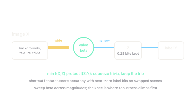
Information theory names the right kept information: a representation $Z$ should minimize what it carries about the input $X$ while maximizing what it carries about the label $Y$ . That compression-versus-prediction tradeoff is the information bottleneck, and it turns "don't learn shortcuts" from a wish into an objective. The probabilistic home is probabilistic foundations; the data-quality ally is data-centric AI.

The one idea you need first. Mutual information $I(A; B)$ measures how much knowing $A$ reduces uncertainty about $B$ , in nats or bits: $I(A;B) = \sum p(a,b)\log\frac{p(a,b)}{p(a)p(b)}$ . Independent variables score zero; perfect predictors score the full entropy. The bottleneck objective is $\min I(X;Z) - \beta I(Z;Y)$ : squeeze the input channel, protect the label channel, with $\beta$ setting the exchange rate.

Think of It Like This

Packing a suitcase for one trip

A good traveler packs everything the trip needs and nothing else: passport, tickets, one adaptable jacket — not the living-room lamp "just in case". Every extra item costs carrying weight; every missing one costs a purchase abroad. The suitcase is judged by the trip, not by how much of home it contains.

A representation is that suitcase. The input image is home with all its clutter (backgrounds, watermarks, scanner brands); the label is the trip. $I(X;Z)$ is the suitcase weight; $I(Z;Y)$ is trip readiness. Shortcut features are lamps: heavy, useless abroad. The bottleneck objective packs deliberately instead of stuffing the whole house.

The analogy stops at the zipper: suitcases have fixed volume, while $\beta$ tunes the tradeoff continuously — and unlike packing, nobody can directly see what got left out.

How It Actually Works

Training optimizes a tractable version of the bottleneck: an encoder $p(z \mid x)$ regularized toward a prior (limiting $I(X;Z)$ ) plus a classifier on $z$ (protecting $I(Z;Y)$ ). The variational bottleneck (VIB) makes both terms computable with the same Gaussian KL machinery as VAEs. InfoMax variants flip the emphasis, maximizing $I(X;Z)$ under augmentation constraints to keep views mutually informative (the engine inside many contrastive methods).

Reading a trained model informationally means probing: accuracy with backgrounds swapped estimates how much $Z$ smuggled, and compression ratios bound how much trivia could hide.

Worked example

A binary feature $Z$ predicts a binary label $Y$ with joint probabilities $P(Z = 0, Y = 0) = 0.4$ , $P(Z = 0, Y = 1) = 0.1$ , $P(Z = 1, Y = 0) = 0.1$ , $P(Z = 1, Y = 1) = 0.4$ .

Margins are uniform ( $0.5$ each), so each cell contributes $p \log(p / 0.25)$ . The $0.4$ cells: $0.4 \times \log(1.6) \approx 0.4 \times 0.470 = 0.188$ each. The $0.1$ cells: $0.1 \times \log(0.4) \approx 0.1 \times (-0.916) = -0.0916$ each. Total: $2 \times 0.188 + 2 \times (-0.0916) = 0.376 - 0.183 = 0.193$ nats, about $0.28$ bits.

So this feature carries $0.28$ bits about the label — modest but real. A shortcut feature scoring high training accuracy with near-zero $I(Z;Y)$ on swapped backgrounds is thereby exposed as memorization.

Code

The point of this snippet is the measurement: mutual information from a contingency table reproduces the $0.193$ nats.

1import math2
3
4def mutual_information(joint: list) -> float:5    total = sum(sum(row) for row in joint)6    rows = len(joint)7    cols = len(joint[0])8    mi = 0.09    for i in range(rows):10        for j in range(cols):11            p = joint[i][j] / total  # joint probability12            pi = sum(joint[i]) / total  # row margin13            pj = sum(joint[r][j] for r in range(rows)) / total  # column margin14            if p > 0:15                mi += p * math.log(p / (pi * pj))16    return mi17
18
19print(round(mutual_information([[0.4, 0.1], [0.1, 0.4]]), 3))  # -> 0.193

Watch Out For

Mutual information is estimated, never measured

In high dimensions MI has no unbiased cheap estimator; variational bounds (MINE, InfoNCE) report lower bounds that move with the estimator's capacity. Teams that read "MI $= 2.1$ " as a physical constant chase estimator artifacts instead of representation changes.

Treat MI numbers as comparisons under one fixed estimator, never as absolutes across papers. If the estimator changes, the scale changes with it.

Beta set once, regretted everywhere

Small $\beta$ over-compresses: features drop label-relevant detail and accuracy sags on hard slices. Large $\beta$ under-compresses: shortcuts survive and robustness never arrives. The failure modes look like opposite problems (underfitting versus overfitting) from one knob.

Sweep $\beta$ across orders of magnitude and plot accuracy against a background-swapped evaluation, not just validation accuracy. The honest setting sits at the knee where robustness climbs before clean accuracy falls.

The Quick Version

Representations should minimize input memory $I(X;Z)$ while protecting label content $I(Z;Y)$ .
The worked fixture computes $0.193$ nats ( $\approx 0.28$ bits) from a $2 \times 2$ joint table.
The bottleneck objective makes the exchange rate explicit through $\beta$ .
High-dimensional MI is a bound under a fixed estimator, not an absolute constant.
Sweep $\beta$ against background-swapped evaluations to find the robustness knee.