Probabilistic and Theoretical Foundations

Vision models guess under uncertainty and must work on images they never saw. Probability and theory supply the language for both: what the model believes, and why it should generalize.

Prior belief plus detector evidence updates to a posterior of 0.82, the shared currency of inference, information, and generalization

Why Does This Exist?

Vision models ship into hospitals and cars while their builders argue about why they work. A detector outputs "cat, 0.9" — is that a calibrated belief or a confident guess? A network trained on a million photos classifies the million-and-first correctly — luck or law? Without theory, every answer is folklore backed by a leaderboard.

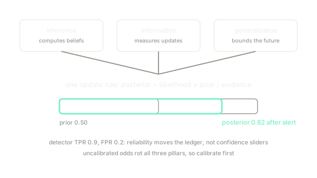
Probability and theory give checkable answers. Approximate inference (variational inference) turns beliefs into computations. Information theory (representation limits) says what features must keep. Generalization theory (bounds) says when training scores predict future ones. This page maps the three pillars and their shared update rule.

The one idea you need first. Bayes' rule updates beliefs with evidence: posterior is proportional to likelihood times prior. In odds language: what you believed, times how much more likely the evidence is under each hypothesis. Every pillar below is this update wearing different clothes — inference computes it, information measures its size, generalization bounds its future error.

Think of It Like This

A betting ledger

A bookmaker opens the day with odds on every horse (the prior). Each race result (evidence) moves the odds: winners shorten, losers lengthen, by exactly the factor the result favors them. The ledger never argues about what "probably" means — it is a number, updated by a rule, settled in cash.

Probabilistic vision keeps the same ledger. The prior says cats appear half the time; the detector's alert is a race result with known reliability; the posterior is the settled odds. Information theory audits how much each result moves the book; generalization theory asks whether today's ledger predicts tomorrow's races. Different questions, one accounting system.

The analogy stops at the stakes: the ledger's odds are calibrated by money, while a network's "0.9" is calibrated only if someone checked — most have not.

How It Actually Works

Three pillars share the update. Approximate inference computes posteriors too complex for closed form: variational methods fit a simple distribution to the true one by optimizing a lower bound. Information theory quantifies the update: mutual information measures how much knowing the features reduces uncertainty about the label, and the bottleneck trades that against compression. Generalization theory bounds the gap between training error and future error using complexity measures (VC dimension, Rademacher averages, PAC-Bayes divergences) that shrink roughly as $1/\sqrt{m}$ with $m$ training samples.

All three assume honest inputs: calibrated likelihoods, representative samples, and a prior you can defend. When those fail, the math still runs and the conclusions quietly rot.

Worked example

A pet camera sees a blurry animal. Prior: $P(\text{cat}) = 0.5$ . The detector alerts "cat" with true-positive rate $0.9$ and false-positive rate $0.2$ . Posterior:

$P(\text{cat} \mid \text{alert}) = \frac{0.9 \times 0.5}{0.9 \times 0.5 + 0.2 \times 0.5} = \frac{0.45}{0.45 + 0.10} = \frac{0.45}{0.55} \approx 0.818$

The alert moves belief from $0.50$ to $0.82$ — a real update with a checkable size. Halve the false-positive rate to $0.1$ and the posterior becomes $0.45 / 0.50 = 0.90$ : reliability, not confidence sliders, drives the result.

Code

The point of this snippet is the update rule both pillars share: plug in reliability numbers and read off the settled belief.

1def posterior(prior: float, tpr: float, fpr: float) -> float:2    hit = tpr * prior  # true alerts3    alarm = hit + fpr * (1.0 - prior)  # all alerts4    return hit / alarm  # Bayes in one line5
6
7print(round(posterior(0.5, 0.9, 0.2), 3))  # -> 0.8188print(round(posterior(0.5, 0.9, 0.1), 3))  # -> 0.9

Watch Out For

Bounds too loose to steer by

Many generalization bounds evaluate to numbers above $1.0$ on real networks — technically true, practically empty. Teams that tune architectures to tighten a vacuous bound optimize a thermometer with no mercury.

Read bounds qualitatively (which terms shrink with data, which grow with complexity) and quantitatively only when the numbers bite below $1$ . A bound that cannot distinguish two models is a compass without a needle.

Uncalibrated odds wearing probability clothes

A softmax "0.9" is not a posterior until calibration is checked — modern networks routinely report $0.9$ while being right $0.7$ of the time. Every downstream update inherits the lie with interest.

Calibrate before propagating: temperature scaling or isotonic regression on held-out data, reliability diagrams as the receipt. Uncertainty you cannot audit is decoration.

The Quick Version

Probability and theory share one update: prior times likelihood, normalized into a posterior.
The worked fixture moves cat belief from $0.50$ to $0.82$ given a detector with $0.9$ TPR and $0.2$ FPR.
Inference computes the update, information theory measures it, generalization bounds its future.
Most published bounds are too loose to rank models; read them for structure, not numbers.
Calibrate likelihoods first, or every pillar inherits confident fiction.