Loss Landscape Analysis

Training walks a mountain range in million-dimensional fog. Loss landscape analysis maps the terrain: sharp ravines that trap, wide valleys that generalize, and the passes between solutions.

A wide valley tolerates shifts that throw a sharp ravine off a cliff, which is why flat minima generalize

Why Does This Exist?

Two networks can share identical training loss and differ wildly on test data. The loss value alone cannot tell a robust solution from a memorized one, yet practitioners must choose checkpoints, tune schedules, and diagnose failures from exactly such numbers. Something has to distinguish good minima from bad ones.

Loss landscape analysis examines the geometry around solutions: curvature (sharp versus flat), barriers between independently trained minima, and how the terrain shifts under distribution change. Flat minima generalize because perturbing them barely moves the loss; connected minima reveal the terrain is one valley system, not isolated pits. The certificate view is PAC-Bayes; the gap view is generalization theory.

The one idea you need first. The Hessian (matrix of second derivatives) measures curvature per direction at a minimum: large eigenvalues mean steep walls, small ones mean flat floors. Sharpness summarizes it — commonly the largest eigenvalue or the loss rise within a small neighborhood. A minimum flat in every direction survives weight jitter and data shift; a sharp one shatters.

Think of It Like This

Camping in a wide valley versus a narrow crack

Two campsites sit at the same altitude. One spreads across a wide valley floor: pitch the tent a meter off and the ground feels identical. The other wedges into a narrow crack: a meter off means a cliff edge or a rock wall. Same elevation, opposite robustness — and when the map shifts (test data differs), the valley camp wakes up fine while the crack camp wakes up falling.

Flat minima are valley floors: quantization, pruning, and distribution shift are all "a meter off", absorbed without damage. Sharp minima are cracks: every perturbation is a cliff. Training loss reports altitude; landscape analysis reports the campsite.

How It Actually Works

Analysts probe geometry three ways. Hessian spectra (via Lanczos approximations, never full matrices) expose curvature scale and outlier directions. Filter-normalized 2-D slices plot loss on a plane through the solution with scale artifacts removed, revealing valley versus ravine shapes. Mode connectivity interpolates linearly between two trained solutions and records the barrier (peak loss along the path): near-zero barriers mean the minima share one connected valley, enabling weight averaging across runs.

Sharpness-aware minimization turns the diagnosis into treatment: it optimizes the worst loss in a neighborhood, explicitly seeking valley floors.

Worked example

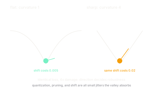
Quadratic bowl $L(w) = 2w_1^2 + 0.5w_2^2$ at point $(1, 1)$ : loss $= 2 + 0.5 = 2.5$ . Hessian is diagonal with entries $4$ and $1$ : curvature $4$ along $w_1$ (sharp), $1$ along $w_2$ (flat). Nudge $0.1$ along each axis and compare loss rises via $\frac{1}{2}\kappa\,\delta^2$ :

Along $w_1$ : $0.5 \times 4 \times 0.01 = 0.02$ .
Along $w_2$ : $0.5 \times 1 \times 0.01 = 0.005$ .

Same step, four times the damage along the sharp axis. A test shift that jitters weights along $w_1$ costs $4\times$ the jitter along $w_2$ — direction, not just distance, decides robustness.

Code

The point of this snippet is the directional damage check: curvature times squared step predicts the rise each axis inflicts.

1def loss_rise(curvature: float, step: float) -> float:2    return 0.5 * curvature * step**2  # second-order rise along one axis3
4
5print(loss_rise(4.0, 0.1))  # -> 0.026print(loss_rise(1.0, 0.1))  # -> 0.005

Watch Out For

Random 2-D slices hide the sharpest directions

A random plane through a million-dimensional minimum almost surely misses its sharpest axes, painting cozy valleys around solutions that are actually ravines. Teams that "visualized the landscape" with one random slice routinely conclude flatness that the Hessian contradicts.

Pair every slice with a Hessian spectrum (or at least top eigenvalues). Slices illustrate; spectra measure. A valley claim needs both.

Sharpness can be gamed by reparameterization

Rescaling layers (multiply one by $10$ , divide the next by $10$ ) leaves the function identical while exploding Hessian eigenvalues. Naive sharpness then screams "ravine" about a valley, and minimizing it distorts the model for a phantom.

Use scale-invariant sharpness (normalized per filter, or adaptive formulations) and sanity-check with actual perturbation tests: jitter weights, quantize, prune slightly. Geometry that vanishes under reparameterization was never terrain.

The Quick Version

Loss value cannot separate robust minima from memorized ones; surrounding geometry can.
The worked fixture shows a $0.1$ step costing $0.02$ along curvature $4$ versus $0.005$ along curvature $1$ .
Flat minima absorb jitter, quantization, and shift; sharp ones amplify them directionally.
Mode connectivity tests whether solutions share a valley: low interpolation barriers enable averaging.
Random slices mislead and raw sharpness games under rescaling, so pair slices with spectra.