Generalization Theory

Training accuracy is a rehearsal; test accuracy is opening night. Generalization theory studies the gap: when rehearsal predicts the show, and what closes the distance.

Test error dips, rises at the interpolation threshold, then dips again as overparameterized models find smoother fits

Why Does This Exist?

Classical wisdom said models with more parameters than samples memorize and fail. Then vision models with millions of parameters fit random labels perfectly — and still classified real photos well. Memorization capacity and good generalization coexisted, which the old story forbade. Either the successes were luck or the story was wrong.

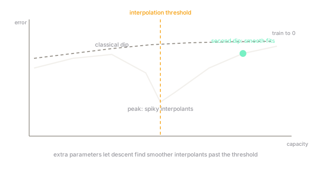
Generalization theory rewrote the story in layers: capacity measures for the small-model regime, double descent for the crossing into overparameterization, and benign overfitting plus inductive bias for why interpolating models pick smooth fits over spiky ones. This page maps those layers with their honest limits. The certificate-flavored layer is PAC-Bayes; the preference-flavored layer is inductive bias.

The one idea you need first. The generalization gap is test error minus training error. Theory bounds or predicts it from three ingredients: how much data ( $m$ ), how complex the model class is (capacity, drift, norms), and how the training procedure searches (implicit bias toward simple fits). No ingredient alone decides; the gap is their argument, and each era of theory foregrounded a different one.

Think of It Like This

Dress rehearsal versus opening night

A theater company rehearses in its own hall for weeks (training) and opens in a new city (test). The rehearsal-to-show gap depends on what was rehearsed: lines memorized word-perfect for one stage crack on another, while acting choices that capture the characters transfer anywhere. Same rehearsal hours, wildly different gaps.

Capacity theory counted rehearsal hours. Modern theory examines the acting: interpolation that memorizes blocking fails, interpolation that captures character generalizes. Double descent is the strange middle where the company first overfits the old hall, then — with far more practice than seems sane — discovers the portable performance underneath.

How It Actually Works

Three regimes stack historically. Classical: test error falls then rises with capacity (U-curve); VC and Rademacher bounds quantify the rise. Double descent: past the interpolation threshold (zero training error), test error falls again as extra parameters let gradient descent find smoother interpolants — the full curve is a separate page (double descent). Benign overfitting: in noisy high dimensions, the minimum-norm interpolant averages noise away, so fitting everything still predicts well. Underneath all three sits inductive bias: gradient descent's preference for simple, smooth, low-frequency fits.

Scale enters through data: gaps typically shrink roughly as $1/\sqrt{m}$ , the same rate behind neural scaling laws.

Worked example

A classifier trains to $0.02$ error and tests at $0.09$ : gap $= 0.09 - 0.02 = 0.07$ . Quadruple the training data (same distribution, same model): the $1/\sqrt{m}$ shape predicts the gap roughly halves, $0.07 / \sqrt{4} = 0.035$ , so test error should land near $0.02 + 0.035 = 0.055$ .

Two honest caveats ride along. First, the shape is asymptotic: small-data behavior wobbles around it. Second, if the extra data comes from a shifted distribution (new cameras, new hospitals), the gap can grow while $m$ grows — the rate assumes representative samples, and reality often declines the assumption.

Code

The point of this snippet is the scaling shape: gaps shrink with the square root of data, which sets expectations before collecting more.

1def expected_gap(gap_now: float, growth: float) -> float:2    return gap_now / (growth**0.5)  # 1/sqrt(m) shape3
4
5print(round(expected_gap(0.07, 4.0), 4))  # -> 0.0356print(round(0.02 + expected_gap(0.07, 4.0), 4))  # -> 0.055

Watch Out For

Test sets that quietly become training sets

Every reuse of the test set for model selection leaks it into training: architecture choices, thresholds, and early stopping all adapt to it. After enough iterations the reported "test" error is a second training error wearing a costume, and the true gap on fresh data surprises everyone.

Lock a final evaluation set early and touch it once, or rotate fresh held-out slices per decision. A gap measured on a negotiated test set measures negotiation skill, not generalization.

Zero training error read as success

Interpolation is now normal, so training error near zero says nothing about which interpolant was found — smooth and portable, or spiky and brittle. Teams that celebrate the zero without probing the fit ship memorizers with excellent dashboards.

Probe the interpolant: background swaps, noise injections, and slice evaluations distinguish smooth fits from spiky ones. The gap lives in those probes long before it reaches the headline metric.

The Quick Version

The generalization gap is test minus training error; theory predicts it from data, complexity, and search bias.
Classical U-curves, double descent past interpolation, and benign overfitting stack historically, not exclusively.
The worked fixture halves a $0.07$ gap to $0.035$ by quadrupling data under the $1/\sqrt{m}$ shape.
Reused test sets become training sets; lock final evaluation early and touch it once.
Zero training error is normal now — probe the interpolant's smoothness instead of celebrating the zero.