PAC-Bayes Bounds

Classical bounds blame model size, yet giant networks generalize. PAC-Bayes bounds blame the distance from initialization instead, which stays small even for huge models.

Training error 0.05 plus a complexity penalty near 0.15 certifies future error below 0.21 in the illustrative bound

Why Does This Exist?

Classical capacity bounds charge by parameter count, and modern vision models carry millions of parameters against tens of thousands of images. The bounds evaluate above $1.0$ — true, vacuous, useless. Yet the models generalize. Something in the classical accounting misprices what training actually does.

PAC-Bayes reprices it. Instead of counting parameters, it measures how far the learned weights travel from where they started, in nats of KL divergence between a posterior and a prior over weights. Training that barely moves (flat regions, good initialization) earns a tight bound regardless of parameter count. The neighboring pages are generalization theory and probabilistic foundations.

The one idea you need first. With probability at least $1 - \delta$ over training samples, the true error of a weight distribution $Q$ is bounded by its training error plus a complexity term shaped like $\sqrt{(KL(Q\,\|\,P) + \log(2\sqrt{m}/\delta)) / (2(m-1))}$ , where $P$ is a fixed prior and $m$ is the sample count. The honest reading is qualitative: error grows with drift-from-prior and shrinks roughly as $1/\sqrt{m}$ . Exact constants below are illustrative arithmetic on that shape, not published tight values.

Think of It Like This

A library fine, not a library census

A library wants to bound how many books go missing. The census approach counts every book on the shelves — millions — and posts a uselessly huge worst case. The ledger approach counts how far books traveled from their slots: borrowed books accrue fines per day away, shelved books cost nothing. A giant library with three books out has a tiny bill.

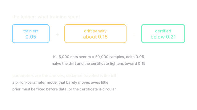
PAC-Bayes is the ledger. Parameters are the shelves; drift from initialization is books-out. A billion-parameter model that training barely moves owes little, while a tiny model dragged across the space owes plenty. Capacity was the wrong thing to count; distance traveled is what training actually spends.

How It Actually Works

Fix a prior $P$ before seeing data (usually centered at initialization). Train to a posterior $Q$ (a distribution around the learned weights, not just the point). Measure training error under $Q$ and the KL divergence $KL(Q\,\|\,P)$ . Plug into the bound: small KL plus low training error certifies low future error. Flat minima help because a wide posterior around a flat minimum stays near the prior while keeping training error low — the same flatness story as loss landscape analysis, now with a certificate.

The prior must be data-free: peeking at training data to center it voids the guarantee silently.

Worked example

Illustrative numbers on the bound's shape: $m = 50{,}000$ samples, training error $0.05$ , $KL(Q\,\|\,P) = 5{,}000$ nats, $\delta = 0.05$ .

Confidence term: $\log(2\sqrt{50{,}000}/0.05) = \log(2 \times 223.6 / 0.05) = \log(8{,}944) \approx 9.1$ .
Complexity: $(5{,}000 + 9.1) / 49{,}999 \approx 0.1002$ .
The bound constrains $kl(0.05 \,\|\, \text{true}) \le 0.1002$ . Inverting numerically, true error $\approx 0.205$ satisfies it (check: $0.05\ln(0.05/0.205) + 0.95\ln(0.95/0.795) \approx -0.0706 + 0.1697 = 0.099 \le 0.1002$ ).

So the certificate reads: future error below about $0.21$ . Halve the drift to $2{,}500$ nats and the bound tightens toward $0.15$ — the ledger rewards staying close to start.

Code

The point of this snippet is the inversion: binary KL solved for the certified error reproduces the $0.205$ bound.

1import math2
3
4def binary_kl(p: float, q: float) -> float:5    return p * math.log(p / q) + (1.0 - p) * math.log((1.0 - p) / (1.0 - q))6
7
8def certify(train_err: float, complexity: float) -> float:9    q = train_err10    while binary_kl(train_err, q) < complexity:  # raise q until KL bites11        q += 0.00112    return round(q, 3)13
14
15print(round(binary_kl(0.05, 0.205), 4))  # -> 0.09916print(certify(0.05, 0.1002))  # -> 0.205

Watch Out For

A prior tuned on training data voids the certificate

Centering the prior at the trained weights, or picking its variance by training performance, spends the data twice. The bound's proof assumes the prior is fixed beforehand; a data-peeking prior makes the certificate circular while the numbers look identical.

Center priors at initialization (or on a held-out split) and freeze them before training. If the "prior" moved after seeing the training set, the bound is decoration.

Huge drift makes the bound vacuous again

Fine-tuning across tasks or long schedules can push $KL(Q\,\|\,P)$ into the millions of nats, and the bound sails past $1.0$ — the same vacuity classical bounds suffered, relocated. The math holds; the certificate says nothing.

Track KL during training as a diagnostic: rising KL with falling training error is normal, but budget it. Data-dependent priors and compression-based bounds exist precisely to rescue drifted regimes.

The Quick Version

PAC-Bayes bounds future error by training error plus drift-from-prior measured in KL nats.
The worked illustration certifies error below about $0.21$ from $0.05$ training error and $5{,}000$ nats of drift.
Flat minima earn tight bounds: wide posteriors stay near the prior without raising training error.
Priors must be fixed before seeing data, or the certificate is circular.
Large drift reintroduces vacuity, so track KL as a training diagnostic.