Object Detection Architectures

Object detectors predict both what is in an image and where it sits, balancing slow two-stage region proposals against fast single-shot dense grids.

Comparing two-stage Faster R-CNN with region proposals against one-stage single-shot detectors like YOLO and RetinaNet.

Why Does This Exist?

Image classification assigns a single categorical label to an entire picture. However, real-world scenes rarely contain a single centered object. Autonomous vehicles must locate multiple pedestrians, cyclists, and traffic signals simultaneously; robotic arms must identify distinct parts scattered across an assembly conveyor.

Early attempts at object localization used a brute-force sliding window approach: an image classifier was evaluated across tens of thousands of cropped bounding boxes at varying spatial scales and aspect ratios. For an image with 50,000 potential bounding boxes, running a deep convolutional network 50,000 times takes several minutes per frame—making real-time vision completely impossible.

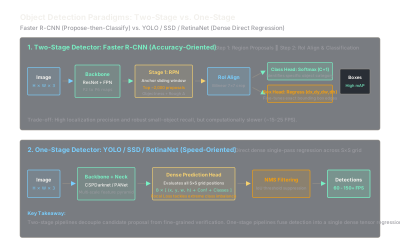
Modern object detection architectures solve this by formulating detection as a unified multitask learning problem that outputs class probabilities alongside spatial coordinate offsets. Modern detectors fall into two dominant paradigms:

Two-Stage Detectors (R-CNN family): First generate category-agnostic candidate region proposals, then crop and classify those specific proposals.
One-Stage Detectors (YOLO, SSD, RetinaNet): Directly regress bounding boxes and class logits across a dense grid in a single forward pass.

Understanding the tension between two-stage precision and one-stage latency is the cornerstone of designing production vision systems.

Think of It Like This

A museum security team vs. a single observant guard

Imagine securing a crowded museum gallery against unauthorized photography.

A two-stage detector operates like a two-person security team. The first guard stands high in the rafters with binoculars (the Region Proposal Network). Their only job is to spot rapid movements or suspicious silhouettes anywhere in the gallery and shout out candidate zones: "Look at bench four! Look at the exit archway!" A second senior guard on the floor walks directly over to those specific zones, confirms whether the person is holding a camera, and determines their exact identity (RoI classification). It is exceptionally thorough and misses few details, but coordinating two guards takes extra time.

A one-stage detector is a single guard equipped with a wide-angle holographic visor. In a single sweeping glance across the room, the guard's visor divides the entire gallery into a geometric grid, predicting the presence, category, and exact perimeter of every person in view simultaneously. It reacts instantaneously at 60 frames per second, but in crowded clusters, the single guard may struggle to distinguish small, overlapping visitors without specialized filtering.

How It Actually Works

The Two-Stage Paradigm: Faster R-CNN

Faster R-CNN (Ren et al., 2015) unified proposal generation and classification onto shared convolutional features:

Backbone + Feature Pyramid Network (FPN): A deep backbone (e.g., ResNet) extracts multi-scale feature maps $\{P_2, P_3, P_4, P_5\}$ , where higher levels capture rich semantics for large objects and lower levels preserve spatial resolution for small objects.
Region Proposal Network (RPN): A small convolutional network slides over each feature map point. At each position, it evaluates $k$ $k$ predefined anchor boxes with varying scales and aspect ratios, predicting:
- Objectness score: $p \in [0, 1]$ (binary foreground vs. background).
- Coordinate delta offsets: $t = (t_x, t_y, t_w, t_h)$ .
RoIAlign: Replaces naive RoI Pooling (which suffered from quantization error when rounding floating-point coordinates to integer grid bins). RoIAlign uses bilinear interpolation at four sampling points per bin to extract fixed-size feature maps ( $7 \times 7$ ) without spatial distortion.
Task Heads: Fully connected layers predict softmax class probabilities over $C + 1$ classes (including background) and fine-tuned bounding box coordinates.

The multitask loss optimizes classification and regression jointly:

\mathcal{L} = \mathcal{L}_{\text{cls}}(p, p^*) + \lambda [p^* \ge 1] \mathcal{L}_{\text{reg}}(t, t^*)

where $\mathcal{L}_{\text{reg}}$ is typically Smooth $L_1$ loss or Generalized IoU (GIoU) loss.

The One-Stage Paradigm: YOLO and RetinaNet

One-stage detectors eliminate the separate proposal step. Models like YOLO (You Only Look Once) divide the input into an $S \times S$ spatial grid. If an object's center falls inside a grid cell, that cell is responsible for detecting it.

Each grid cell predicts $B$ bounding box tuples:

\text{Prediction} = \left[ x, y, w, h, \text{Confidence}, \text{Class}_1, \ldots, \text{Class}_C \right]

Historically, one-stage detectors suffered from lower accuracy on small objects due to extreme foreground-background class imbalance: a dense grid produces over 100,000 candidate locations per image, of which fewer than 10 contain real objects. Normal cross-entropy is overwhelmed by easy negative background examples.

RetinaNet solved this using Focal Loss:

\text{FL}(p_t) = -\alpha_t (1 - p_t)^\gamma \log(p_t)

The modulating factor $(1 - p_t)^\gamma$ (with $\gamma = 2.0$ ) dynamically downweights well-classified background examples ( $p_t \to 1$ ), focusing gradient updates on difficult, ambiguous foreground objects.

Non-Maximum Suppression (NMS)

Because one-stage and two-stage detectors predict multiple overlapping boxes for a single object, Non-Maximum Suppression post-processes the detections:

Sort candidate boxes by classification confidence score.
Select the box $B_{\text{max}}$ with the highest confidence.
Compute Intersection-over-Union (IoU) with all remaining candidates:

\text{IoU}(A, B) = \frac{\text{Area}(A \cap B)}{\text{Area}(A \cup B)}

Suppress and discard any box where $\text{IoU} \ge \text{threshold}$ (typically 0.5 to 0.7).
Repeat for the next unsuppressed candidate.

Worked Example

Let us calculate the Intersection-over-Union (IoU) between a predicted bounding box $A$ and a ground-truth box $B$ :

Box $A$ : $[x_1=50, y_1=50, x_2=150, y_2=150]$ (width = 100, height = 100)
Box $B$ : $[x_1=100, y_1=100, x_2=200, y_2=200]$ (width = 100, height = 100)

Compute individual areas:

\text{Area}(A) = 100 \times 100 = 10\text{,}000, \quad \text{Area}(B) = 100 \times 100 = 10\text{,}000

Compute intersection box coordinates:

\begin{aligned} x_{\text{int\_left}} &= \max(50, 100) = 100, \quad y_{\text{int\_top}} = \max(50, 100) = 100 \\ x_{\text{int\_right}} &= \min(150, 200) = 150, \quad y_{\text{int\_bottom}} = \min(150, 200) = 150 \end{aligned}

Intersection width: $150 - 100 = 50$
Intersection height: $150 - 100 = 50$

\text{Area}(A \cap B) = 50 \times 50 = 2\text{,}500

Compute union area:

\text{Area}(A \cup B) = \text{Area}(A) + \text{Area}(B) - \text{Area}(A \cap B) = 10\text{,}000 + 10\text{,}000 - 2\text{,}500 = 17\text{,}500

Compute IoU:

\text{IoU}(A, B) = \frac{2\text{,}500}{17\text{,}500} = \frac{1}{7} \approx 0.1429

Since $\text{IoU} \approx 0.143 < 0.5$ , NMS would consider these two boxes non-overlapping and would not suppress either.

Code

1import torch2
3def compute_iou(boxes_a: torch.Tensor, boxes_b: torch.Tensor) -> torch.Tensor:4    """Compute pairwise Intersection-over-Union (IoU) between bounding box sets.5    Boxes format: [x1, y1, x2, y2]6    """7    # Intersection coordinates8    inter_x1 = torch.max(boxes_a[:, 0], boxes_b[:, 0])9    inter_y1 = torch.max(boxes_a[:, 1], boxes_b[:, 1])10    inter_x2 = torch.min(boxes_a[:, 2], boxes_b[:, 2])11    inter_y2 = torch.min(boxes_a[:, 3], boxes_b[:, 3])12
13    inter_w = (inter_x2 - inter_x1).clamp(min=0.0)14    inter_h = (inter_y2 - inter_y1).clamp(min=0.0)15    inter_area = inter_w * inter_h16
17    # Areas18    area_a = (boxes_a[:, 2] - boxes_a[:, 0]) * (boxes_a[:, 3] - boxes_a[:, 1])19    area_b = (boxes_b[:, 2] - boxes_b[:, 0]) * (boxes_b[:, 3] - boxes_b[:, 1])20    union_area = area_a + area_b - inter_area21
22    return inter_area / union_area.clamp(min=1e-6)23
24# Test with our worked example tensors:25box_a = torch.tensor([[50.0, 50.0, 150.0, 150.0]])26box_b = torch.tensor([[100.0, 100.0, 200.0, 200.0]])27
28iou = compute_iou(box_a, box_b)29print(round(iou.item(), 4))30# -> 0.1429

Watch Out For

Coordinate parametrization drift and NMS occlusion blind spots

When training custom bounding box heads, practitioners frequently parametrize box offsets directly as absolute pixel values $[x, y, w, h]$ . This causes unstable training because coordinate gradients scale with image resolution. Instead, always use log-space and normalized anchor offsets:

t_x = \frac{x - x_a}{w_a}, \quad t_y = \frac{y - y_a}{h_a}, \quad t_w = \log\left(\frac{w}{w_a}\right), \quad t_h = \log\left(\frac{h}{h_a}\right)

Furthermore, standard greedy NMS can accidentally delete real objects in dense crowds (such as two pedestrians standing directly in front of each other, where their boxes have $\text{IoU} > 0.5$ ). When deploying detectors in high-density scenes, switch to Soft-NMS (which decays scores with a Gaussian penalty instead of hard deletion) or modern end-to-end transformer-based heads that avoid NMS entirely.

The Quick Version

Two-stage detectors (Faster R-CNN) prioritize localization accuracy and small-object detection by separating region proposals from classification.
One-stage detectors (YOLO, SSD) prioritize inference throughput, predicting class scores and box offsets in a single unified dense pass.
RoIAlign uses bilinear interpolation to eliminate the quantization misalignment bugs of older RoI Pooling.
Focal Loss stabilizes one-stage detector training by suppressing the gradient contribution of massive numbers of easy background samples.
Non-Maximum Suppression (NMS) removes redundant overlapping predictions by iteratively pruning bounding boxes based on IoU overlap thresholds.