Optimal Transport
Comparing two clouds of pixels needs the cheapest way to morph one into the other. Optimal transport finds that morphing plan, and its cost is a distance that respects geometry.
Why Does This Exist?
Classic divergences go blind exactly when generators need them most. KL divergence between disjoint supports is infinite (or saturates), so a generator placing all mass slightly off the data gets the same "terrible" as one placing it miles away — no gradient, no direction, no learning. Pixel-wise losses have the opposite flaw: shifting an image by one pixel costs as much as scrambling it.
Optimal transport (OT) measures the cheapest way to morph one distribution into the other, priced by a ground cost (usually Euclidean distance). Nearby-but-disjoint distributions get small distances with live gradients, which is why Wasserstein GANs stabilized adversarial training. The probabilistic home is probabilistic foundations; the compression-versus-content sibling is information theory.
The one idea you need first. A transport plan says how much mass moves from each supply point to each demand point. The Wasserstein distance is the minimum total cost over all valid plans: mass times distance, summed. The plan itself is useful output — it matches samples across domains, aligns histograms, and pairs generated images with real ones for evaluation.
Think of It Like This
Wheelbarrows of dirt
Two piles of dirt must become two new piles elsewhere. Hire wheelbarrows: every load moved one meter costs one coin. The foreman's plan lists which old pile feeds which new pile; the bill is loads times meters, summed. The cheapest valid plan is the optimal transport cost.
KL divergence is a foreman who only asks whether dirt exists at each spot and charges infinity for any new location — useless while the piles differ. Pixel loss charges per wheelbarrow regardless of distance — a meter and a mile cost the same. Only the wheelbarrow bill respects the geometry of the move, which is why generators trained on it walk toward the data instead of teleporting or stalling.
How It Actually Works
The Kantorovich formulation optimizes over joint distributions (plans) with the two distributions as marginals: every supply unit assigned, every demand unit filled, cost minimized. For discrete distributions this is a linear program; entropy regularization (Sinkhorn) makes it fast and differentiable at the price of slight blur. In vision, OT aligns color histograms for style transfer, matches feature distributions for domain adaptation, and scores generators (Fréchet-style distances approximate Wasserstein-2 on Gaussian-fitted features).
The 1-D special case is beautifully simple: the optimal plan matches sorted quantiles, so Wasserstein distance is the area between cumulative curves.
Worked example
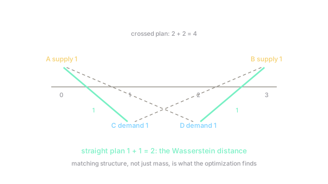
Supply: unit at position (pile A), unit at position (pile B). Demand: unit at position (hole C), unit at position (hole D). Ground cost is absolute distance.
Candidate plan 1 (straight): A→C costs ; B→D costs . Total .
Candidate plan 2 (crossed): A→D costs ; B→C costs . Total .
No other valid plan exists for single units, so the Wasserstein-1 distance is . Note the crossed plan costs double for the same endpoints — matching structure, not just mass, is what the optimization discovers.
Code
The point of this snippet is the plan comparison: enumerate the two matchings and read off the minimum as the distance.
import itertools
def plan_cost(assign: tuple, supply: list, demand: list) -> float: return sum(abs(s - demand[d]) for s, d in zip(supply, assign))
supply, demand = [0, 3], [1, 2]costs = {p: plan_cost(p, supply, demand) for p in itertools.permutations([0, 1])}print(costs) # -> {(0, 1): 2, (1, 0): 4}print(min(costs.values())) # -> 2Watch Out For
Exact OT scales cubically and bites at batch size
Exact solvers run roughly , so matching thousands of samples per batch is hopeless. Teams that prototype on hundreds of points and "scale up later" discover the later never comes.
Use entropic regularization (Sinkhorn, near-quadratic with a good epsilon) for training loops, and reserve exact solvers for small evaluation sets. Report the regularization strength alongside the number — it biases the distance downward.
The ground cost decides the answer
Wasserstein with pixel Euclidean cost calls a shifted image far; with perceptual-feature cost it calls it near. Same distributions, different distances, different model rankings. The metric inherits whatever the ground cost believes about similarity.
Choose the ground cost deliberately (perceptual features for natural images, spatial distance for layouts) and state it with every reported number. An OT score without its ground cost is uninterpretable.
The Quick Version
- Optimal transport prices the cheapest morph between distributions; that price is the Wasserstein distance.
- The worked fixture gives straight-plan cost versus crossed-plan , so the distance is .
- Unlike KL, it stays finite with live gradients on disjoint supports, stabilizing generator training.
- Exact solvers scale cubically, so training uses Sinkhorn regularization with reported strength.
- The ground cost determines the answer, so pair the number with the cost that produced it.