Pooling and Downsampling

Pooling summarizes each small patch of a feature map into one value, trading exact positions for cheaper maps and sturdier features.

A 2 by 2 max-pooling window keeps only the strongest activation per patch, halving each side of a 4 by 4 map.

Why Does This Exist?

A 1080p frame at $1920 \times 1080$ with $32$ float32 channels costs $1920 \times 1080 \times 32 \times 4 = 265{,}420{,}800$ bytes, about $265$ MB for one feature map, before any batch or gradient. Running every later layer at full resolution is unaffordable, and exact pixel positions are often noise: a classifier should fire whether the tire sits ten pixels left or right. Pooling compresses each local patch into one value, halving spatial sides per step while keeping the strongest signals. Two stride-2 steps shrink that $265$ MB map $16$ -fold to about $16.6$ MB. This page covers window pooling and its learned cousin, strided convolution. What flows through the windows is taught in feature maps, and the stride arithmetic in padding and stride.

Think of It Like This

Judging a choir by section

A judge scores a choir split into sections. For each section the judge writes down one number: with max-pooling it is the loudest singer's volume, with average-pooling it is the section's overall hum. Swapping two singers inside one section changes nothing on the score sheet.

The window is the section, the stride is how sections tile the stage, and swap-proof scores are translation invariance. The analogy stops at seating: the judge still remembers where each section sat, but pooling forgets exact positions. Tasks that need locations, like drawing boxes or masks, must recover them elsewhere.

How It Actually Works

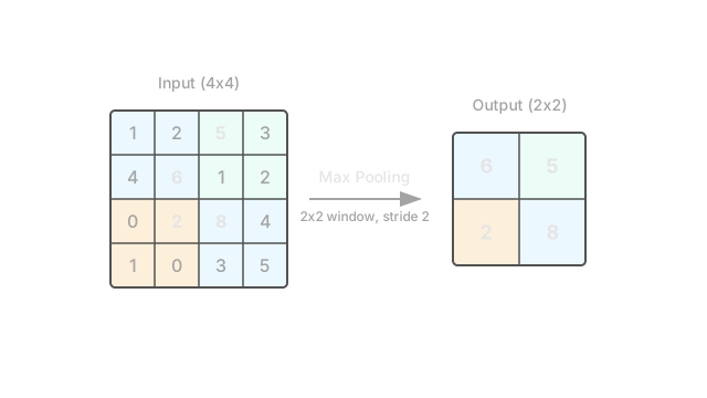
A pooling layer slides a $K \times K$ window with stride $S$ over each channel independently, where $K$ is the window side and $S$ is the step between windows. The output side is $\lfloor (W - K)/S \rfloor + 1$ for input side $W$ , so $K = 2$ and $S = 2$ halves each side and quarters the values. Max pooling outputs $y = \max_{i \in R}(x_i)$ over window $R$ , keeping the strongest activation and killing the rest, which suits sparse signals like edges. Average pooling outputs $y = \frac{1}{|R|} \sum_{i \in R} x_i$ , smoothing the patch, which suits texture and density but dilutes a lone strong spike. Global average pooling pushes this to the limit: one value per channel for the whole map, feeding the classifier with no dense layer. Strided convolution instead steps its learned kernel with $S = 2$ , downsampling with weights the network tunes rather than a fixed rule.

Worked 4 by 4 example

Input rows $[1, 3, 2, 4]$ , $[5, 6, 1, 2]$ , $[0, 1, 8, 7]$ , $[3, 2, 4, 5]$ with $K = 2$ , $S = 2$ give output side $\lfloor (4 - 2)/2 \rfloor + 1 = 2$ . The top-left window $[1, 3, 5, 6]$ max-pools to $6$ and averages to $(1 + 3 + 5 + 6)/4 = 3.75$ . Scoring all four windows gives max output rows $[6, 4]$ and $[3, 8]$ , and average output rows $[3.75, 2.25]$ and $[1.5, 6.0]$ .

Code

1img = [2    [1.0, 3.0, 2.0, 4.0],3    [5.0, 6.0, 1.0, 2.0],4    [0.0, 1.0, 8.0, 7.0],5    [3.0, 2.0, 4.0, 5.0],6]7
8def pool(img, fn):9    out = []10    for r in (0, 2):11        row = []12        for c in (0, 2):13            window = [img[r + dr][c + dc] for dr in (0, 1) for dc in (0, 1)]14            row.append(fn(window))15        out.append(row)16    return out17
18print(pool(img, max))19# -> [[6.0, 4.0], [3.0, 8.0]]20
21def mean(xs):22    return sum(xs) / len(xs)23
24print(pool(img, mean))25# -> [[3.75, 2.25], [1.5, 6.0]]

Watch Out For

Pooling away the resolution a locator needs

Classification survives heavy downsampling, but detectors and segmenters read positions off the map. The symptom is vanished small objects and blobby masks after a total stride of $32$ on tiny inputs. Budget the strides across the backbone, and recover detail with skip connections or dilated convolutions instead of stacking more pools.

Average-pooling a sparse signal map

When only a few cells carry the defect, edge or spike, averaging divides it by the whole window. The symptom is a strong $9.0$ spike inside a $2 \times 2$ window of zeros scoring $2.25$ and missing its threshold. Use max pooling for sparse presence signals and reserve averaging for texture, density and tail summaries.

The Quick Version

Pooling summarizes each $K \times K$ patch into one value with stride $S$ between windows.
A $2 \times 2$ stride-2 pool halves each side and quarters the value count.
Max pooling keeps the strongest activation; average pooling smooths the patch.
Example: the $4 \times 4$ map above max-pools to rows $[6, 4]$ and $[3, 8]$ .
Global average pooling collapses each channel to one value for the classifier.
Strided convolution downsamples with learned weights instead of a fixed rule.