Basic CNN Operations

Convolutions slide small weight templates across an image to spot local patterns, while strides, padding, and pooling govern how feature maps shrink.

2D convolution sliding over a feature map with padding and stride, alongside max pooling spatial downsampling.

Why Does This Exist?

Fully connected multilayer perceptrons fail on high-resolution image data. If you feed an uncompressed $1024 \times 1024$ color image with 3 channels into a standard dense hidden layer with 1,024 units, that single linear projection requires over 3.2 billion weight parameters ( $1024 \times 1024 \times 3 \times 1024 \approx 3.22 \times 10^9$ ). Storing those floats demands roughly 12.8 gigabytes of RAM for one layer, leading to immediate memory exhaustion and devastating overfitting.

Dense layers also treat pixel positions as completely independent coordinates. If an edge or object shifts five pixels to the right, a fully connected network views that shifted image as a completely new input pattern and must relearn the visual cue from scratch.

Basic convolutional operations solve this by enforcing two inductive biases: local connectivity and translation equivariance. Instead of connecting every pixel to every neuron, a convolutional filter scans local neighborhoods with shared weights. Strides, padding, and pooling operations give practitioners precise mathematical control over spatial resolution, receptive field growth, and computational throughput.

Think of It Like This

A magnifying glass stamp and a photo album summary

Imagine inspecting a large mosaic wall through a small $3 \times 3$ frosted magnifying tile. As you slide the tile across each square of the mosaic, you multiply the tile's colored lens tints against the mosaic tiles underneath and jot down a single score representing how well that patch matches the pattern. Sliding the same small tile across every row and column ensures you spot an identical pattern whether it appears in the top-left corner or bottom-right corner.

Padding is the foam border you attach around the edges of the wall so your magnifying tile can center directly over the edge tiles without falling off. Stride is how many tiles you hop each time you slide your magnifying glass. Finally, pooling is like replacing every group of four detailed field notes with just the highest or average score to make the photo album lighter to carry.

How It Actually Works

Discrete 2D Cross-Correlation and Dimension Arithmetic

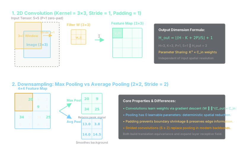
In deep learning frameworks, the forward convolution layer actually implements the discrete cross-correlation operator. For an input tensor $X \in \mathbb{R}^{C_{\text{in}} \times H \times W}$ and a learnable filter bank $W \in \mathbb{R}^{C_{\text{out}} \times C_{\text{in}} \times K_h \times K_w}$ with bias $b \in \mathbb{R}^{C_{\text{out}}}$ , the activation at output channel $c_{\text{out}}$ and spatial coordinate $(i, j)$ is:

Y[c_{\text{out}}, i, j] = b[c_{\text{out}}] + \sum_{c=0}^{C_{\text{in}}-1} \sum_{m=0}^{K_h-1} \sum_{n=0}^{K_w-1} X[c, i \cdot S_h + m - P_h, j \cdot S_w + n - P_w] \cdot W[c_{\text{out}}, c, m, n]

where $S$ represents the stride step size, $P$ represents the zero-padding added to each border, and $K$ represents kernel spatial size.

The spatial output dimensions $H_{\text{out}}$ and $W_{\text{out}}$ follow exact discrete floor arithmetic:

H_{\text{out}} = \left\lfloor \frac{H_{\text{in}} - K_h + 2P_h}{S_h} \right\rfloor + 1, \quad W_{\text{out}} = \left\lfloor \frac{W_{\text{in}} - K_w + 2P_w}{S_w} \right\rfloor + 1

When using standard square filters ( $K_h = K_w = K$ , $P_h = P_w = P$ , $S_h = S_w = S$ ):

Valid padding ( $P=0$ ): No padding added. The output shrinks by $K - 1$ pixels per dimension when $S=1$ .
Same padding ( $P = (K - 1) / 2$ for odd $K$ and $S=1$ ): Output spatial dimensions exactly equal input spatial dimensions ( $H_{\text{out}} = H_{\text{in}}$ ).
Downsampling stride ( $S \ge 2$ ): Skips locations, cutting spatial resolution roughly by a factor of $S$ .

Spatial Pooling Mechanics

Pooling layers slide an aggregation window across the spatial grid without learnable parameters:

Max Pooling: Takes $\max_{(m,n)} X[c, i \cdot S + m, j \cdot S + n]$ . Retains the strongest activation (e.g., sharp edge or textured feature) while providing small translation invariance.
Average Pooling: Computes $\frac{1}{K_h K_w} \sum_{(m,n)} X[c, i \cdot S + m, j \cdot S + n]$ . Smoothes activations across the receptive field, frequently used as Global Average Pooling (GAP) before classifier heads.

Worked Example

Let us trace a single-channel $4 \times 4$ input matrix $X$ convolved with a $3 \times 3$ kernel $K$ , with stride $S=1$ and padding $P=0$ :

X = \begin{bmatrix} 1 & 2 & 0 & 1 \\ 0 & 3 & 1 & 2 \\ 2 & 1 & 0 & 2 \\ 1 & 0 & 3 & 1 \end{bmatrix}, \quad K = \begin{bmatrix} 1 & 0 & -1 \\ 1 & 0 & -1 \\ 1 & 0 & -1 \end{bmatrix}, \quad b = 0

Determine output shape:

H_{\text{out}} = \left\lfloor \frac{4 - 3 + 2(0)}{1} \right\rfloor + 1 = 2, \quad W_{\text{out}} = 2

The output $Y$ is a $2 \times 2$ matrix.

Compute top-left cell $Y[0, 0]$ (receptive field $X[0:3, 0:3]$ ):

\begin{aligned} Y[0, 0] &= (1 \cdot 1 + 2 \cdot 0 + 0 \cdot (-1)) + (0 \cdot 1 + 3 \cdot 0 + 1 \cdot (-1)) + (2 \cdot 1 + 1 \cdot 0 + 0 \cdot (-1)) \\ &= (1 + 0 + 0) + (0 + 0 - 1) + (2 + 0 + 0) = 1 - 1 + 2 = 2 \end{aligned}

Compute top-right cell $Y[0, 1]$ (receptive field $X[0:3, 1:4]$ ):

\begin{aligned} Y[0, 1] &= (2 \cdot 1 + 0 \cdot 0 + 1 \cdot (-1)) + (3 \cdot 1 + 1 \cdot 0 + 2 \cdot (-1)) + (1 \cdot 1 + 0 \cdot 0 + 2 \cdot (-1)) \\ &= (2 - 1) + (3 - 2) + (1 - 2) = 1 + 1 - 1 = 1 \end{aligned}

Compute bottom-left cell $Y[1, 0]$ (receptive field $X[1:4, 0:3]$ ):

\begin{aligned} Y[1, 0] &= (0 \cdot 1 + 3 \cdot 0 + 1 \cdot (-1)) + (2 \cdot 1 + 1 \cdot 0 + 0 \cdot (-1)) + (1 \cdot 1 + 0 \cdot 0 + 3 \cdot (-1)) \\ &= (-1) + (2) + (1 - 3) = -1 + 2 - 2 = -1 \end{aligned}

Compute bottom-right cell $Y[1, 1]$ (receptive field $X[1:4, 1:4]$ ):

\begin{aligned} Y[1, 1] &= (3 \cdot 1 + 1 \cdot 0 + 2 \cdot (-1)) + (1 \cdot 1 + 0 \cdot 0 + 2 \cdot (-1)) + (0 \cdot 1 + 3 \cdot 0 + 1 \cdot (-1)) \\ &= (3 - 2) + (1 - 2) + (-1) = 1 - 1 - 1 = -1 \end{aligned}

Final convolution output:

Y = \begin{bmatrix} 2 & 1 \\ -1 & -1 \end{bmatrix}

If we now apply $2 \times 2$ Max Pooling over $Y$ with stride $S=2$ , the single output value is $\max(2, 1, -1, -1) = 2$ .

Code

1import torch2import torch.nn as nn3
4# Define an input tensor: Batch=1, Channels=1, Height=4, Width=45x = torch.tensor([[[[1.0, 2.0, 0.0, 1.0],6                    [0.0, 3.0, 1.0, 2.0],7                    [2.0, 1.0, 0.0, 2.0],8                    [1.0, 0.0, 3.0, 1.0]]]], dtype=torch.float32)9
10# Construct 2D Convolution: 1 in_channel, 1 out_channel, 3x3 kernel, no bias11conv = nn.Conv2d(in_channels=1, out_channels=1, kernel_size=3, stride=1, padding=0, bias=False)12
13# Assign hand-computed vertical edge detection weights14weight = torch.tensor([[[[1.0, 0.0, -1.0],15                         [1.0, 0.0, -1.0],16                         [1.0, 0.0, -1.0]]]], dtype=torch.float32)17with torch.no_grad():18    conv.weight.copy_(weight)19
20out_conv = conv(x)21print(out_conv.shape)22# -> torch.Size([1, 1, 2, 2])23print(out_conv.squeeze().tolist())24# -> [[2.0, 1.0], [-1.0, -1.0]]25
26# Apply 2x2 Max Pooling with stride 227pool = nn.MaxPool2d(kernel_size=2, stride=2)28out_pool = pool(out_conv)29print(out_pool.squeeze().item())30# -> 2.0

Watch Out For

Asymmetric padding mismatches causing unaligned feature coordinates

When applying an even kernel size (such as $2 \times 2$ or $4 \times 4$ ) with "same" padding, integer division $(K - 1) / 2$ yields a fraction. Frameworks like TensorFlow and PyTorch handle this differently: PyTorch's padding=1 on a $2 \times 2$ kernel adds 1 pixel symmetrically on both sides, yielding $H_{\text{out}} = H_{\text{in}} + 1$ , whereas TensorFlow's padding="SAME" pads asymmetrically (more on the right/bottom than left/top).

This discrepancy shifts receptive field centers, causing spatial misalignment when importing pre-trained weights between PyTorch and ONNX/TensorFlow or concatenating feature pyramid maps. Always prefer odd kernel sizes ( $3 \times 3$ , $5 \times 5$ , $7 \times 7$ ) so symmetric padding $P = (K - 1) / 2$ preserves perfect integer spatial alignment centered on each pixel.

The Quick Version

Convolutions extract visual features via sliding local receptive fields with shared parameter weights.
Output spatial resolution obeys $H_{\text{out}} = \lfloor (H_{\text{in}} - K + 2P)/S \rfloor + 1$ .
Odd kernel sizes ( $3 \times 3$ , $5 \times 5$ ) allow clean, symmetric zero-padding to keep feature map resolutions intact.
Pooling provides non-parametric spatial downsampling; max pooling preserves prominent edges while average pooling captures regional intensity.
Modern architectures often replace pooling layers with stride-2 convolutions to let the network learn optimal downsampling filters.