Pose Estimation

Pose estimation finds body joints as image points and links them into a skeleton, turning pixels into a structure that reveals action.

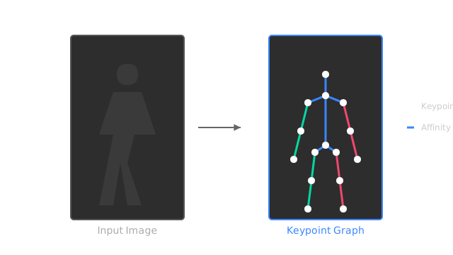
One heatmap per joint peaks at its pixel, and linking the peaks builds the skeleton that reveals the action.

Why Does This Exist?

Detecting a person says someone is present; it cannot say whether they are running, waving or falling. Pixels carry clothing, lighting and clutter that action classifiers must ignore. Pose estimation compresses the figure into a skeleton: named joints such as elbows and knees plus the limbs between them, a low-dimensional structure where a raised arm is visible as moved points rather than changed pixels. This page covers 2D joint prediction: heatmap outputs, the top-down and bottom-up pipelines, and the similarity score that judges them. Lifting flat skeletons into depth lives in 3D human pose estimation, rigid-object rotation and translation in 6D pose estimation, and the classic multi-person system in OpenPose.

Think of It Like This

Pinning a puppet to a corkboard

Trace a dancer onto a corkboard by pushing one pin per joint: shoulders, elbows, wrists, hips, knees, ankles. String connects the pins into limbs. To check whether the dancer waves, you watch the wrist pin, not the whole board.

The pins are keypoints, the string is the skeleton graph, and the board clutter you ignore is background pixels. The analogy stops at hiding: a pin behind the board is simply gone, while a model must decide per joint whether it is visible or guessed, and a wrong guess bends the whole puppet.

How It Actually Works

Networks rarely regress $(x, y)$ coordinates directly. For each of $J$ joints the network outputs one heatmap $H_j$ over the image grid, where each cell holds the probability that joint $j$ sits at that pixel, and the prediction is the argmax cell. Heatmaps suit convolutional learning because a wrong-but-near peak still gives useful gradient, while a single coordinate number gives none. Top-down pipelines detect each person first, crop the box, and run single-person estimation per crop: accurate, but cost grows per person. Bottom-up pipelines predict all joints of each type at once over the full frame, then group them into skeletons with learned tags or part-affinity fields: one network pass for crowds, with grouping errors when bodies overlap.

Worked heatmap and OKS example

A $4 \times 4$ wrist heatmap peaks at $0.9$ in row $1$ , column $2$ , so the joint is heatmap pixel $(x, y) = (2, 1)$ , or $(8, 4)$ input pixels at stride $4$ . Accuracy uses Object Keypoint Similarity: for visible joints, $\text{OKS} = \sum_i \exp(-d_i^2 / (2 s^2 k_i^2)) / n$ , where $d_i$ is the pixel error of joint $i$ , $s$ is the person scale in pixels, $k_i$ is a per-joint constant, $n$ counts visible joints, and invisible joints are skipped. Take an ankle with $d = 5$ , $s = 200$ , $k = 0.089$ : the exponent is $-25 / (2 \times 200^2 \times 0.089^2) = -25 / 633.68 = -0.0395$ , so that joint scores $\exp(-0.0395) = 0.9613$ , nearly perfect despite a five-pixel miss.

Code

1heat = [2    [0.1, 0.2, 0.1, 0.0],3    [0.2, 0.5, 0.9, 0.3],4    [0.0, 0.3, 0.4, 0.1],5    [0.0, 0.1, 0.0, 0.0],6]7cells = [(v, r, c) for r, row in enumerate(heat) for c, v in enumerate(row)]8value, r, c = max(cells)9print((value, r, c))10# -> (0.9, 1, 2)11print((c * 4, r * 4))12# -> (8, 4)13
14import math15
16d, s, k = 5.0, 200.0, 0.08917print(round(math.exp(-(d ** 2) / (2 * s ** 2 * k ** 2)), 4))18# -> 0.9613

Watch Out For

Hallucinating joints under occlusion

Hidden legs and cropped torsos have no pixels, yet the network must output something per joint. The symptom is confident skeletons with knees pinned onto desks and doorframes. Gate every joint on its peak confidence and mark weak peaks invisible instead of linking them, since one invented joint bends the whole graph.

Reading jittery argmax peaks as motion

Two plausible peaks near a hand, or a flat plateau, make the argmax hop between neighboring cells frame to frame. The symptom is a resting wrist vibrating by several pixels in the track. Shift the peak a quarter pixel toward the second maximum for sub-pixel stability, then smooth tracks over time before deriving velocity.

The Quick Version

Pose estimation turns figures into joint-plus-limb skeletons that reveal action.
Networks output one probability heatmap per joint and take each peak as the position.
Example: a $0.9$ peak at row $1$ , column $2$ is pixel $(8, 4)$ at stride $4$ .
Top-down crops each person first; bottom-up predicts all joints once, then groups.
OKS scores predictions with tolerance scaled by person size and joint type.
A five-pixel ankle miss at scale $200$ still scores $0.9613$ .