Replay Methods for Continual Vision
Mix a small buffer of old images into every new batch, so the gradient sees the old task again and stops overwriting it.
Why Does This Exist?
Catastrophic forgetting happens because the new batch contains zero old examples, so the gradient has no old-task term. The most direct repair is to put old examples back into the batch. Keep a buffer of earlier images, sample from it every step, and train on the mixture. The gradient then genuinely optimizes both.
It is the baseline every fancier method must beat. Regularization without data in regularization methods and separate parameters in architecture methods both justify themselves against this number. The parent framing is continual learning.
Think of It Like This
Rehearsing old songs at every practice
A band learns a new set list but opens every rehearsal by replaying three old songs. The new songs still get most of the evening, yet fingers never lose the old ones because they are played weekly. The buffer is the rehearsal shortlist: too small and rare songs vanish, recency-only and the old hits age out. The analogy stops at interference: songs share little fingering, while image classes share features, so mixing old images changes what the new ones learn too.
How It Actually Works
Each training step draws part of the batch from new data and part from the buffer, typically around half and half. The loss is the sum over the mixed batch, so backpropagation carries both terms. Variants differ only in what the buffer holds: raw images, compressed features, or a generator that synthesizes old-looking examples when retention rules forbid storage.
Worked example with recomputed numbers
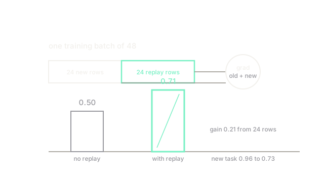
Use the same 20-feature probe as the forgetting page. Task A accuracy after plain B training is 0.50. Build each B batch of 48 as 24 new B rows plus 24 kept A rows, reusing the same 24 A rows across steps. After 600 steps old accuracy reads 0.71, a gain of 0.21 from 24 stored rows, while new-task accuracy lands at 0.73 instead of 0.96. Doubling kept rows to 48 lifts old accuracy to about 0.79 in this setup, with diminishing returns past one full representative per class group.
Sampling decides what survives
Fill the buffer by recency and rare classes vanish first, exactly the classes where a mistake costs most. Keep it class balanced with a floor of examples per class, or score rows by loss contribution and keep the informative ones. Count examples per class against what the model must still do, then enforce that count every stage.
Watch Out For
A buffer that silently becomes recent-only
Reservoir sampling over a stream converges to mostly recent classes, and old accuracy for rare classes falls quarters later with no code change. The symptom is per-class old accuracy fanning out while the mean looks acceptable. Fix it with explicit per-class quotas and a quarterly count audit against the quota.
Storing images the policy forbids keeping
Faces, plates, and medical frames often carry deletion duties that make raw buffers unlawful, and the violation surfaces at audit time, not training time. Check retention before choosing raw replay. When storage is barred, use feature replay, generative replay, or regularization, and record which one the policy forced.
The Quick Version
- Replay puts old examples into every new batch, restoring the missing gradient term directly.
- In the worked probe, 24 kept rows lift old accuracy from 0.50 to 0.71.
- The new task pays for it, here 0.96 down to 0.73, which is the visible trade.
- Buffer policy is the method: class-balanced quotas beat recency sampling.
- When raw storage is barred, use feature or generative replay instead of breaking retention rules.