Spiking Neural Networks

Ordinary neurons output numbers every tick; spiking neurons stay silent until voltage crosses threshold, then fire. Computation becomes events in time, not arithmetic in layers.

Voltage climbs with leak, crosses threshold at step two, fires once, and resets, encoding strength as timing

Why Does This Exist?

Dense networks multiply everything by everything, every tick — billions of multiply-accumulates dominated by zeros and near-zeros. Brains pay per spike instead: silent neurons cost nothing, active ones cost a blip. For always-on vision that gap is the difference between a wall plug and a coin cell.

Spiking neural networks (SNNs) compute with spike events in time. Leaky integrate-and-fire (LIF) neurons accumulate inputs, leak toward rest, fire on crossing threshold, and reset — turning intensity into spike rate or timing. They run natively on event streams and neuromorphic chips. The hardware home is neuromorphic vision; the sensor feed is event cameras.

The one idea you need first. A LIF neuron updates in discrete ticks: $V \leftarrow V + \text{input} - \text{leak}$ , then if $V \ge \theta$ it emits a spike and resets (to rest or by subtraction). Strong input fires fast, weak input leaks away unfired. Information lives in rate (spikes per window) or timing (first-spike latency), never in a floating activation.

Think of It Like This

A bucket with a leak and a bell

Each neuron is a bucket under dripping inputs, with a small hole leaking constantly and a bell that rings when water tops the rim — then the bucket empties. Heavy drip (strong input) rings fast; drizzle evaporates through the leak unheard. The network's message is the pattern of bells, not water levels.

Ordinary networks measure everyone's water level every second, full census. Spiking networks listen for bells. The leak is memory with a half-life (recent drips matter, old ones drained); the threshold is attention (only full buckets speak). Computation becomes listening, and listening is cheap.

How It Actually Works

Forward passes simulate LIF dynamics over tens of ticks: spikes propagate as binary events, and downstream neurons integrate them through weights — accumulation without multiplication, since spikes are $0/1$ . Training takes two roads: surrogate gradients replace the spike's zero-derivative with a smooth proxy during backprop (straight-through style), or ANN-to-SNN conversion trains conventionally then maps activations to firing rates with calibrated thresholds. Readouts count spikes, race first spikes, or vote across populations.

Temporal coding (timing carries the message) is efficient and finicky; rate coding (counts carry it) is robust and slow. Most vision SNNs mix both.

Worked example

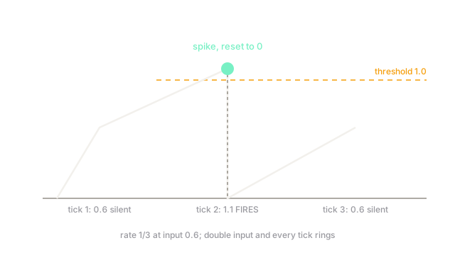
One LIF neuron, rest $0$ , leak $0.1$ per tick, threshold $\theta = 1.0$ , constant input $0.6$ per tick:

Tick 1: $V = 0 + 0.6 - 0 = 0.6$ (no leak from rest on the first fill; equivalently $0 + 0.6$ ). Below threshold: silent.
Tick 2: $V = 0.6 + 0.6 - 0.1 = 1.1 \ge 1.0$ : SPIKE. Reset to $0$ .
Tick 3: $V = 0 + 0.6 = 0.6$ : silent.

One spike in three ticks: rate $1/3 \approx 0.33$ . Double the input to $1.2$ and tick 1 alone reaches $1.2 \ge 1.0$ — rate $1.0$ . Strength becomes timing, monotonically and without a single multiplication at inference.

Code

The point of this snippet is the bucket: leak, threshold, reset, and counted bells reproduce the worked trace.

1def lif_trace(inputs: list, leak: float = 0.1, theta: float = 1.0) -> list:2    v, spikes = 0.0, []3    for x in inputs:  # one tick per input4        v = v + x - (leak if v > 0 else 0.0)5        if v >= theta:6            spikes.append(1)7            v = 0.0  # reset after ringing8        else:9            spikes.append(0)10    return spikes11
12
13print(lif_trace([0.6, 0.6, 0.6]))  # -> [0, 1, 0]14print(sum(lif_trace([1.2, 1.2, 1.2])))  # -> 3

Watch Out For

The spike's derivative is zero almost everywhere

Spikes are step functions: flat (derivative $0$ ) except at the threshold where it is undefined. Naive backprop sends no learning signal at all — networks sit untrained while loss curves flatline innocently.

Surrogate gradients (smooth stand-ins active near threshold) restore learning but bias it; conversion sidesteps training spikes entirely. Either way, validate that trained weights actually use timing — dead-neuron audits (neurons that never fire) catch surrogate collapse early.

Conversion latency buys accuracy with time

ANN-to-SNN conversion reaches parity only with long simulation windows (tens to hundreds of ticks): rate codes need time to resolve fine values. Short windows quantize activations coarsely and accuracy sags exactly where the deployment wanted speed.

Budget ticks like bits: more ticks, finer rates, slower answers. Match the window to the accuracy target up front instead of discovering the tradeoff in production.

The Quick Version

SNNs compute with threshold-crossing spikes: silent neurons cost nothing, bells carry messages.
The worked fixture fires $[0, 1, 0]$ on steady $0.6$ input with leak $0.1$ and threshold $1.0$ .
Strength encodes as rate or timing; inference needs accumulation, not multiplication.
Surrogate gradients or ANN conversion train through the zero-derivative steps.
Audit for dead neurons, and budget simulation ticks against accuracy before deploying.