SRCNN

SRCNN proved three small convolutional layers can learn upscaling end to end, replacing hand-built pipelines with patch extraction, mapping, and rebuild.

Why Does This Exist?

Super-resolution pipelines were hand-assembled: bicubic upscale, sparse-code each patch against a learned dictionary, average overlaps. Every stage was tuned separately and errors compounded opaquely. The sparse-coding step especially was slow iterative optimisation per patch.

SRCNN collapsed the pipeline into three convolutional layers trained jointly: $9 \times 9$ patch extraction with $64$ filters, $1 \times 1$ nonlinear mapping with $32$ filters, $5 \times 5$ reconstruction. It beat the state of the art immediately and ran feed-forward fast. The task framing is super-resolution, and the perceptual successor is ESRGAN.

Think of It Like This

Three specialists on an assembly line

An old workshop routes every chair through separate shops: cutting, joinery, finishing, each with its own foreman and its own tolerances. SRCNN merges the shops into one line of three stations under a single foreman who sees only finished chairs.

Joint training is the single foreman: the extraction filters learn what the mapping needs, not what looks interpretable alone. The line fails when one station cannot express its job, three thin layers cap the complexity any single stage can hold, which deeper successors fixed.

How It Actually Works

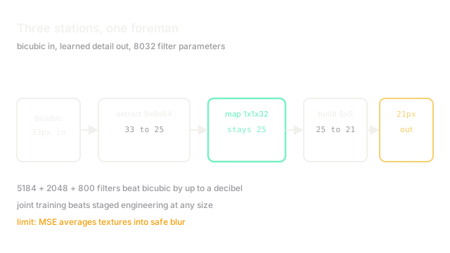
Input is the bicubic-upscaled low-resolution image. Layer one extracts overlapping patches: $64$ filters of $9 \times 9$ turn each neighbourhood into a $64$ -number description. Layer two maps descriptions nonlinearly: $32$ filters of $1 \times 1$ mix channels per position. Layer three rebuilds: one $5 \times 5$ filter (three for colour) assembles the high-resolution output. Loss is plain MSE against ground truth.

With valid convolutions, a $33 \times 33$ training patch shrinks $33 - 9 + 1 = 25$ , stays $25$ through $1 \times 1$ , then $25 - 5 + 1 = 21$ , so each sample supervises a $21 \times 21$ output. Filters total $9^2 \times 64 + 64 \times 32 + 32 \times 5^2 \approx 8{,}000$ parameters, tiny by any modern standard.

Worked example

Parameter count: $81 \times 64 = 5{,}184$ in layer one, $64 \times 32 = 2{,}048$ in layer two, $32 \times 25 = 800$ in layer three, total $8{,}032$ plus biases. Training on $91$ images with millions of sampled patches, this pocket model gained roughly $0.5$ – $1.0$ dB over bicubic on standard benchmarks, the first proof that joint learning beats staged engineering for upscaling.

Code

Receptive arithmetic that sizes training patches to outputs.

1def srcnn_output(patch: int = 33) -> int:2    """Output size after 9-1-5 valid convolutions."""3    h = patch - 9 + 1  # extraction shrinks the patch4    h = h - 1 + 1  # 1x1 mapping preserves size5    return h - 5 + 1  # reconstruction shrinks again6
7
8print(srcnn_output())  # -> 21 output pixels per 33 input9print(81 * 64 + 64 * 32 + 32 * 25)  # -> 8032 filter parameters

Watch Out For

MSE training that guarantees safe blur

SRCNN optimises squared error, so it outputs the average of plausible details. Edges stay clean but textures wash out, the safe-blur signature of every MSE upscaler.

Accept SRCNN outputs as fidelity baselines, not perceptual champions. For visual sharpness move to adversarial or perceptual losses.

Border shrinkage mishandled at test time

Valid convolutions shrink outputs, so naive tiling misaligns assembled images by the lost border. Stitch tiles without accounting and seams grid the result.

Pad inputs or crop consistently so assembly matches training geometry. Test full-image assembly, not just centre crops.

The Quick Version

SRCNN replaces staged sparse-coding pipelines with three jointly trained convolutions.
Filters run $9 \times 9 \times 64$ , then $1 \times 1 \times 32$ , then $5 \times 5$ reconstruction.
$33$ -pixel patches yield $21$ -pixel outputs through valid convolutions.
About $8{,}032$ filter parameters beat bicubic by up to a decibel.
MSE training blurs textures, and border geometry needs care at assembly.