Variational Inference

Exact Bayesian answers need impossible integrals. Variational inference picks a simple family of guesses and tunes the closest member, turning integration into optimization.

The approximate posterior sits close to the prior at a KL cost of 1.25 nats, the price the ELBO pays for data fit

Why Does This Exist?

Bayesian vision wants posteriors over millions of weights or latent codes, and the normalizing integral has no closed form. Sampling (MCMC) is exact in the limit and glacial in practice — nobody runs full MCMC on a vision transformer. The field needed posterior-ish answers at optimization speed.

Variational inference (VI) reframes the integral as an optimization: choose a tractable family (usually Gaussians), then find the member closest to the true posterior by maximizing a lower bound on the evidence. VAEs, Bayesian compression, and countless latent-variable vision models train on exactly this bound. The framework it lives in is probabilistic foundations; the gradient-based cousin is score matching.

The one idea you need first. The ELBO (evidence lower bound) splits into two pulls: $\text{ELBO} = \mathbb{E}_q[\log p(x \mid z)] - KL(q(z) \,\|\, p(z))$ . The first term rewards reconstructions that explain the image; the second charges rent for drifting from the prior. Maximizing the ELBO tightens a guaranteed lower bound on $\log p(x)$ , so better bounds mean better models with a certificate attached.

Think of It Like This

A cookie cutter for a cloud

A pastry chef must reproduce a cloud shape in dough, but cutters come only in ellipses. She tries ellipses of every center and width, keeps the one overlapping the cloud best, and accepts the leftover mismatch as the price of using a cutter at all.

VI is that fitting. The cloud is the true posterior; the ellipse drawer is the Gaussian family; the overlap score is the negative KL divergence. A richer cutter set (mixtures, flows) fits better and costs more, and no ellipse ever becomes a cloud — the family you choose caps what you can catch.

How It Actually Works

Pick $q(z)$ (mean-field Gaussian is the default), write the ELBO, and ascend its gradient: the reconstruction term flows through the reparameterization trick ( $z = \mu + \sigma \epsilon$ with $\epsilon$ fixed noise, so gradients reach $\mu$ and $\sigma$ ), while the KL term is often closed-form for Gaussian pairs. At convergence $q$ is the family's best portrait of the posterior, and the ELBO value lower-bounds the model's evidence for comparison across architectures.

For two one-dimensional Gaussians $q = \mathcal{N}(\mu, \sigma^2)$ and $p = \mathcal{N}(0, 1)$ , the price of drifting is closed-form: $KL = \log(1/\sigma) + (\sigma^2 + \mu^2)/2 - 1/2$ .

Worked example

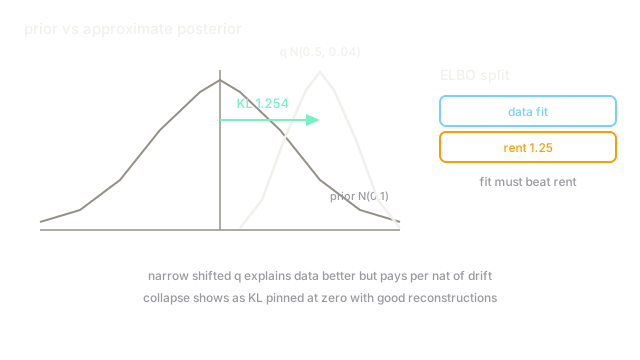
Approximate a 1-D posterior with $q = \mathcal{N}(\mu = 0.5,\ \sigma = 0.2)$ against prior $\mathcal{N}(0, 1)$ :

Scale term: $\log(1 / 0.2) = \log 5 \approx 1.609$ .
Drift term: $(0.04 + 0.25) / 2 = 0.29 / 2 = 0.145$ .
Constant: $-0.5$ .
Total: $KL \approx 1.609 + 0.145 - 0.5 = 1.254$ nats.

The narrow, shifted Gaussian costs $1.25$ nats of rent. The ELBO then reads: reconstruction log-likelihood minus $1.25$ . If the data fit improves by less than that, the optimizer drags $q$ back toward the prior — the bound automatically distrusts overconfident drift.

Code

The point of this snippet is the rent calculation: closed-form Gaussian KL reproduces the worked $1.254$ exactly.

1import math2
3
4def gaussian_kl(mu: float, sigma: float) -> float:5    return math.log(1.0 / sigma) + (sigma**2 + mu**2) / 2.0 - 0.56
7
8print(round(gaussian_kl(0.5, 0.2), 3))  # -> 1.2549print(round(gaussian_kl(0.0, 1.0), 3))  # -> 0.0

Matching the prior exactly costs zero, as it must; the shifted narrow guess costs $1.254$ nats.

Watch Out For

KL direction seeks one mode and hides the rest

VI minimizes $KL(q \,\|\, p)$ , which punishes $q$ for covering regions where $p$ is tiny but barely punishes missing whole modes of $p$ . The fitted Gaussian locks onto one posterior mode and reports full confidence, blind to the others.

For multimodal posteriors (ambiguous images!), widen the family with mixtures or treat VI uncertainty as a lower bound on true uncertainty. A single Gaussian's confidence over a forked posterior is a fiction the loss function endorses.

Posterior collapse in VAEs

When the decoder is powerful, the ELBO's optimum sets $q(z \mid x)$ equal to the prior for every $x$ : KL hits zero, reconstruction ignores the latents, and the "generative model" generates without using its code. The loss looks fine while the representation dies.

Watch the KL term per dimension during training — collapse shows as KL pinned at zero while reconstructions stay good. Weaken the decoder, anneal the KL weight up from zero, or use free-bits floors per latent group.

The Quick Version

VI replaces intractable posterior integrals with optimization over a simple distribution family.
The ELBO trades reconstruction fit against KL rent to the prior; both terms are checkable.
The worked fixture prices a shifted narrow Gaussian at $1.254$ nats of KL.
$KL(q \,\|\, p)$ is mode-seeking, so single-Gaussian fits understate uncertainty on ambiguous inputs.
In VAEs, watch for posterior collapse: zero KL with good reconstructions means dead latents.