Visual Servoing

Visual servoing steers a robot by watching features move in the image, driving them toward desired positions instead of following blind trajectories.

Feature error in the image drives velocity commands that shrink the error to zero

Why Does This Exist?

Preplanned arm motions fail when the mug shifts 2 cm mid-reach. Blind trajectories cannot see the shift. Visual servoing exists to close that gap: watch the target continuously and convert image error into velocity right now. The robot homes onto moving or miscalibrated targets instead of replaying a plan that assumed a static world.

For tracking features see object tracking and for motion see optical flow.

Think of It Like This

Backing a car into a parking line using mirrors

You do not memorize wheel angles. You watch the line drift in the mirror and steer to shrink the gap until it centers. Faster drift means faster wheel. Visual servoing is that mirror loop with math: image error in, joint velocity out. The analogy stops at mirrors: robots also model how each joint moves each feature.

How It Actually Works

Current features $s$ and desired features $s^*$ define error $e = s - s^*$ . Here $s$ may hold point coordinates, line parameters, or moments. An interaction matrix $L$ maps camera velocity to feature motion. The control law $v = -\lambda L^+ e$ commands velocity proportional to error, where $\lambda$ sets speed and $L^+$ is the pseudoinverse. Image-based servoing compares in pixels and tolerates calibration error. Position-based servoing estimates 3D pose first and commands in space, which tracks straighter paths when calibration is excellent.

Worked example

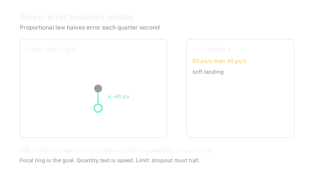
A point sits at $(320, 200)$ with goal $(320, 240)$ , so $e = (0, -40)$ pixels. With $\lambda = 2$ per s and unit interaction, commanded vertical speed is $80$ pixels per s toward the goal. After 0.25 s the point reaches $(320, 220)$ and error halves to $-20$ , so speed halves to $40$ pixels per s. The exponential slowdown lands softly instead of overshooting, which is the signature of proportional servoing.

Code

This snippet servos a point to its goal.

1import numpy as np2
3
4def servo(s: np.ndarray, goal: np.ndarray, lam: float = 2.0, dt: float = 0.05) -> np.ndarray:5    traj = [s.copy().astype(float)]6    for _ in range(10):7        e = traj[-1] - goal8        v = -lam * e9        traj.append(traj[-1] + v * dt)10    return np.round(np.array(traj), 1)11
12
13t = servo(np.array([320.0, 200.0]), np.array([320.0, 240.0]))14print(t[0].tolist(), t[5].tolist(), t[-1].tolist())  # -> [320.0, 200.0] [320.0, 216.4] [320.0, 226.1]

Error decays geometrically. Larger $\lambda$ hurries but risks oscillation on noisy features.

Watch Out For

Lost features that drive blind

Occlusion or motion blur drops the tracked points and the error freezes at its last value, so the arm keeps driving on stale evidence. The symptom is confident motion toward empty space. The fix monitors feature count and covariance, halts or re-acquires below threshold, and never integrates error through dropout.

The Quick Version

Servoing maps image error directly to velocity commands.
Proportional control gives exponential convergence without overshoot.
Image-based control tolerates calibration error; pose-based needs it exact.
Feature loss must halt motion, not freeze the last error.
Tune speed against noise; fast gains oscillate on blur.