VQ-VAE

VQ-VAE compresses an image into a grid of discrete codebook tokens instead of smooth numbers, giving generators a finite vocabulary of visual words.

Why Does This Exist?

Continuous latents are awkward for the strongest generators. Transformers predict discrete tokens, words, IDs, and a smooth Gaussian vector gives them nothing to classify. Researchers wanted the scaling power of next-token prediction applied to images, but images have no vocabulary.

Vector quantisation builds one. By forcing every encoder output through a finite codebook of learned visual words, VQ-VAE turns a photo into a sentence of token IDs. That discrete grid is exactly what powers autoregressive image models, as the owner page autoregressive image generation shows from the generator side. The continuous alternative it departs from is the variational autoencoder.

Think of It Like This

A paint-by-numbers kit with 512 mixed colours

A paint shop holds millions of blendable shades. A paint-by-numbers kit offers 512 premixed pots and a rule: every region of your painting must use the nearest premixed colour. The finished picture is coarser than a freehand blend, but anyone can reproduce it exactly by reading out pot numbers, and a machine can learn to predict those numbers one region at a time.

The codebook is the kit. Quantisation error is the visible gap between the shade you wanted and the nearest pot. It fails when the kit misses a colour family entirely, whole skies collapse into one pot, which is the codebook collapse pitfall below.

How It Actually Works

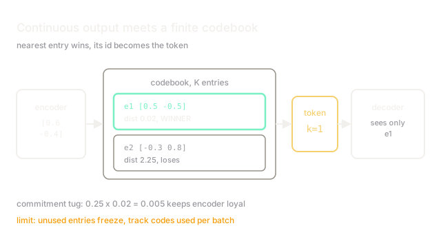
The encoder outputs a continuous vector $z_e(x)$ per spatial location. A codebook holds $K$ learned vectors $e_1, \dots, e_K$ , usually $K = 512$ . Quantisation snaps each output to its nearest entry:

k = \arg\min_j \lVert z_e(x) - e_j \rVert_2, \qquad z_q = e_k

The decoder only ever sees $z_q$ . Gradients cannot flow through the $\arg\min$ , so training copies decoder gradients straight through to the encoder, the straight-through estimator, and moves codebook vectors toward the encoder outputs assigned to them with a separate dictionary loss. A third term, the commitment loss $\beta \lVert z_e(x) - \mathrm{sg}[e_k] \rVert^2$ with $\beta \approx 0.25$ , keeps the encoder loyal to its chosen entry instead of drifting between codes. The symbol $\mathrm{sg}$ means stop-gradient: that term trains the encoder only.

Worked example

Encoder output $z_e = [0.6, -0.4]$ . Codebook has $e_1 = [0.5, -0.5]$ and $e_2 = [-0.3, 0.8]$ . Distances squared: to $e_1$ , $(0.1)^2 + (0.1)^2 = 0.02$ ; to $e_2$ , $(0.9)^2 + (-1.2)^2 = 0.81 + 1.44 = 2.25$ . Nearest is $e_1$ , so the region becomes token $k = 1$ and the decoder receives exactly $[0.5, -0.5]$ . Commitment loss is $0.25 \times 0.02 = 0.005$ , a gentle tug keeping the encoder near its pick.

Code

Nearest-code lookup plus the commitment term, the heart of the forward pass.

1def quantize(z_e: list[float], codebook: list[list[float]], beta: float = 0.25) -> tuple:2    """Snap encoder output to nearest code; return token, vector, commitment loss."""3    dists = [sum((a - b) ** 2 for a, b in zip(z_e, e)) for e in codebook]4    k = min(range(len(dists)), key=dists.__getitem__)5    return k, codebook[k], beta * dists[k]6
7
8z_e = [0.6, -0.4]9book = [[0.5, -0.5], [-0.3, 0.8]]10print(quantize(z_e, book))  # -> (1, [0.5, -0.5], 0.005)

Watch Out For

Codebook collapse leaves most entries unused

Early in training a few entries win every lookup, get all the gradient, and win more, while hundreds of codes sit frozen. Reconstructions then reuse a tiny visual vocabulary and look posterised.

Track the fraction of codes used per batch. If it drops under half, restart dead entries near active encoder outputs or use exponential moving-average codebook updates, which spread assignments far more evenly than plain gradient steps.

Expecting smooth interpolation between tokens

In a continuous latent space, averaging two codes gives a sensible in-between image. Token IDs have no arithmetic: the average of token $1$ and token $9$ is not token $5$ in any meaningful sense.

Interpolate in encoder space before quantisation, or decode both endpoints and blend pixels. Never blend IDs.

The Quick Version

VQ-VAE replaces each continuous encoder output with its nearest learned codebook vector.
The image becomes a grid of discrete token IDs, a vocabulary transformers can predict.
Gradients bypass the lookup via straight-through estimation while a dictionary loss moves the codes.
Our example snaps $[0.6, -0.4]$ to token $1$ at distance $0.02$ with commitment cost $0.005$ .
Watch for dead codebook entries and never interpolate raw token IDs.