Core ML

Variational Autoencoders

A plain autoencoder's latent space has holes, so sampling it gives nothing. Make the encoder emit a distribution instead of a point and the gaps fill in.

The encoder emits a mean and a spread rather than a point, a separate standard-normal sample enters from outside, and combining them is what leaves a differentiable path back through the sampling step

Why Does This Exist?

A ceramics studio has 4,000 photographs of vase silhouettes going back sixty years, and the design team wants twenty new ones by Monday. Not copies, not blends of two chosen pots. New shapes that look like they belong.

An autoencoder gets close. It squeezes each silhouette down to eight numbers and rebuilds it faithfully, so those eight numbers evidently hold what a vase is. Feed the decoder eight numbers of your own and you should get a vase.

You get noise. Every time.

That's the wall, and it isn't a bug. Nothing during training asked the encoder to use the space between the silhouettes it saw. It scattered 4,000 codes wherever was convenient and the decoder only learned what to do at those spots. Pick a point at random and you've landed in a void.

So the fix is about the space, not the decoder. Two words first: a latent space is where those codes live, and a divergence measures how far one distribution sits from another — KL divergence here.

Think of It Like This

Pinning butterflies against spraying them

A collector pins 4,000 butterflies to a board, each at one exact spot. Precise, and the board is mostly bare cork. Point anywhere between two pins and you're pointing at nothing.

Now do it differently. For each butterfly, spray a soft patch of paint centred where the pin would have gone, wide enough that neighbouring patches overlap. The board fills in, every point inside somebody's patch, so every point means something.

Two pressures decide the patch size, pulling opposite ways. To keep the butterflies distinguishable you want patches small and far apart; to leave no bare cork, broad and overlapping. Where those settle is a board you can point at blind and still hit a butterfly.

How It Actually Works

Two terms, permanently in tension

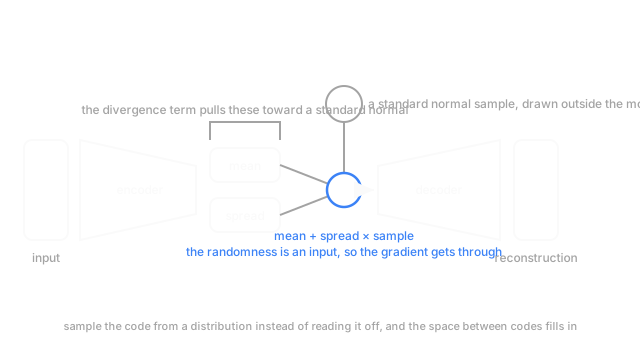
The encoder stops emitting a code. It emits a mean and a spread, one pair per latent dimension, and the code is drawn from that distribution. The loss gains a second term:

\mathcal{L} = \underbrace{\lVert x - \hat{x} \rVert^2}_{\text{reconstruction}} + \underbrace{D_{\mathrm{KL}}\!\left(q(z \mid x) \,\|\, p(z)\right)}_{\text{keep the patches spread out}}

$x$ is the silhouette, $\hat{x}$ the rebuild, $q(z \mid x)$ the distribution the encoder produced for it, and $p(z)$ a standard normal — the shape you want the whole board to take.

Those two terms are the collector's two pressures. Reconstruction wants each vase's patch narrow and far from the others, so codes stay distinguishable. The divergence term wants every patch centred at the origin with unit width, so they overlap and fill the space. Neither wins — what you get is organised and continuous, which is what makes sampling work: draw eight numbers from a standard normal, decode, land inside the region the decoder was trained on.

The trick that makes it trainable

There's a hole in that story. Training needs gradients to reach the encoder, and there's now a sampling step in the way. You can't differentiate through "draw a number at random".

The reparameterisation trick moves the randomness out of the path. Instead of sampling from the encoder's distribution, sample $\epsilon$ from a standard normal outside the model, then compute

z = \mu + \sigma \epsilon

Identical distribution. Completely different graph. Now $\epsilon$ is an input, like the image, and $z$ is an ordinary differentiable function of $\mu$ and $\sigma$ , so the derivative of anything downstream flows straight back through. That's the accented join in the diagram, and the single move the method rests on.

What it cost

Reconstructions come out blurry. Squared error on pixels rewards the average of everything that could plausibly have been there, and the average of several sharp edges is soft. That is the loss behaving correctly, not the model failing.

And you now have a term that can win outright. If the divergence pressure overwhelms reconstruction, the encoder gives up and returns the standard normal for every input — the patches merge and the board carries no information. That failure has a name, below.

A VAE optimises a bound on the data's likelihood, so it has an explicit if approximate density. GANs never write a probability down.

Show Me the Code

The trick, measured. Both routes estimate the same derivative; only one is cheap enough to train with.

1import numpy as np2
3rng = np.random.default_rng(0)4MU, SIGMA, N = 1.5, 0.7, 100_0005
6
7def decoder_loss(z: np.ndarray) -> np.ndarray:8    return z ** 2  # a stand-in for whatever the decoder charges for a code9
10
11eps = rng.normal(0.0, 1.0, N)12z = MU + SIGMA * eps  # the noise is an input now, so the derivative of z by mu is just 113reparam = 2.0 * z  # chain rule straight through the sample14score = decoder_loss(z) * (z - MU) / SIGMA ** 2  # no path, so estimate it from scratch15print(f"exact           {2 * MU:.4f}")16print(f"reparameterised {reparam.mean():.4f}   spread {reparam.std() / np.sqrt(N):.4f}")17print(f"score function  {score.mean():.4f}   spread {score.std() / np.sqrt(N):.4f}")18# -> exact           3.000019# -> reparameterised 2.9987   spread 0.004420# -> score function  2.9925   spread 0.0222

Both land on 3.0, so both are valid. The spread is the story: five times noisier without the trick, from the same 100,000 samples. Multiply that noise across millions of parameters and training stops working.

Watch Out For

Posterior collapse, where the divergence term wins

The symptom is oddly cheerful. Total loss falls nicely, the divergence term drops to near zero, and reconstructions are decent. Then you sample and every draw decodes to roughly the same vase.

The encoder has stopped reading its input. It returns the standard normal for every silhouette, the divergence term is satisfied perfectly, and a strong decoder carries reconstruction alone by memorising an average pot. Watch the divergence term as its own number, not inside the total: a healthy run holds it clearly above zero. Both standard fixes weaken the pressure temporarily — ramp the divergence weight up from zero over the first few thousand steps, or hold it below a floor so the encoder is never rewarded for going silent.

Sampling from the encoder instead of from the prior

Generation code that reads an image, takes the encoder's mean and spread, samples, decodes. Lovely output, and it generated nothing — those are variations on a silhouette you already had, which is what an autoencoder with noise does.

Sample from the prior, the standard normal, with no input image anywhere in the call. That's the only version that tests whether the space actually filled in. The wrong way round hides the exact failure you needed to catch, because a model with a half-empty latent space still reconstructs beautifully.

The Quick Version

A plain autoencoder's latent space has voids, so decoding a point you never encoded returns nothing. This page is the fix.
The encoder emits a mean and a spread per dimension instead of a code, sampled from that.
The loss gains a divergence term pulling every distribution toward a standard normal, fighting reconstruction on purpose. That tension fills the space.
Sampling blocks gradients, so reparameterise: draw the noise outside the model and compute mean plus spread times noise. The derivative flows straight through.
Squared-error reconstruction averages over plausible outputs, which is why samples come out soft.
If the divergence term wins outright the encoder ignores its input. Watch that term separately, and sample from the prior when you evaluate.