3D Gaussian Splatting

Instead of querying a dense neural network for every light ray, represent a 3D scene as millions of fuzzy colored ellipsoids and splat them directly onto the camera lens.

Anisotropic 3D Gaussians are projected via viewing Jacobians to 2D screen splats and composited using tile-based alpha blending.

Why Does This Exist?

Neural Radiance Fields (NeRFs) proved that neural networks could synthesize photorealistic novel views of complex real-world scenes. However, NeRFs require evaluating a multi-layer perceptron dozens or hundreds of times along every individual camera ray. At $1920 \times 1080$ resolution, rendering a single image requires hundreds of millions of forward passes through a neural network, limiting frame rates to fractions of a frame per second and requiring hours or days of compute to optimize.

Traditional point clouds render fast, but raw points leave holes and cannot model view-dependent specularity or semi-transparent boundaries. Triangle meshes struggle to capture complex geometries like hair, foliage, and diffuse reflections without heavy manual cleanup.

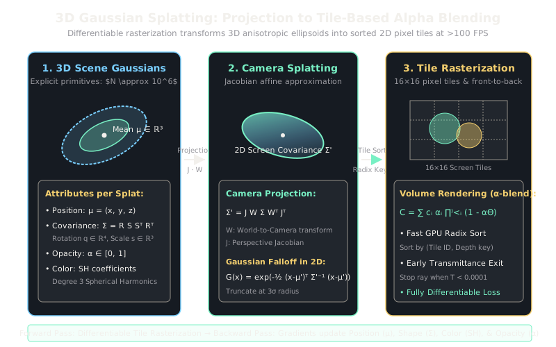
3D Gaussian Splatting (3DGS) replaces implicit neural ray marching with explicit, differentiable volumetric primitives. By defining a scene as millions of parameterized 3D Gaussians and projecting them directly onto screen tiles using a custom GPU rasterizer, 3DGS achieves equal or superior visual fidelity to NeRFs while training in minutes and rendering at over 100 frames per second.

Think of It Like This

A cloud of colored spray-paint droplets against glass

Imagine recreating a sculpture by suspending millions of tiny, translucent droplets of colored spray paint in mid-air. Each droplet has a specific position, a stretched oval shape, an orientation, an opacity, and a color that slightly shifts depending on where you stand.

To see what the sculpture looks like from any angle, you hold a clear glass pane in front of it and press the droplets flat against the glass surface. Droplets in front cover up droplets behind them according to their transparency. Rather than examining the entire depth of the room point by point, you simply stamp the overlapping colored patches onto the glass in order from front to back.

How It Actually Works

Differentiable Projection and Covariance Formulation

A 3D Gaussian is centered at mean $\mu \in \mathbb{R}^3$ and defined by a 3D covariance matrix $\Sigma$ :

G(x) = \exp\left(-\frac{1}{2} (x - \mu)^T \Sigma^{-1} (x - \mu)\right)

Because a valid covariance matrix must be positive semi-definite, direct gradient descent on $\Sigma$ is prone to invalid configurations. 3DGS decomposes $\Sigma$ into a scaling vector $s \in \mathbb{R}^3$ and a rotation quaternion $q \in \mathbb{R}^4$ :

\Sigma = R S S^T R^T

where $S = \text{diag}(s)$ is a diagonal scaling matrix and $R$ is the orthonormal rotation matrix derived from normalized quaternion $q$ .

To render these 3D Gaussians from a camera view defined by viewing transform $W$ and projective transformation, the 3D covariance is projected into a 2D screen-space covariance $\Sigma'$ using the local affine Jacobian $J$ of the projective transformation:

\Sigma' = J W \Sigma W^T J^T

Each Gaussian carries an opacity $\alpha \in [0, 1]$ and view-dependent color coefficients $c$ represented via spherical harmonics (SH) up to degree 3.

During rendering, the screen is subdivided into $16 \times 16$ pixel tiles. The rasterizer discards Gaussians outside the viewing frustum (or beyond a $99\%$ confidence radius of $3\sigma$ ). The remaining Gaussians are assigned 64-bit keys containing their tile ID and view depth, sorted rapidly via GPU radix sort, and alpha-blended front-to-back:

C = \sum_{i \in \mathcal{N}} c_i \alpha_i \prod_{j=1}^{i-1} (1 - \alpha_j)

Rasterization terminates early when accumulated opacity reaches $1 - \epsilon$ (typically transmittance $T < 0.0001$ ), avoiding needless compute for occluded splats.

Worked Example

Consider a single 3D Gaussian positioned at camera coordinates $\mu = [0, 0, 2]^T$ with focal length $f_x = f_y = 500$ pixels and optical center at the origin $(0, 0)$ .

Affine Jacobian $J$ at depth $z = 2$ : The perspective projection maps $[x, y, z]^T \to [f_x x / z, f_y y / z]^T$ . The Jacobian evaluated at $\mu = [0, 0, 2]^T$ is:
$J = \begin{bmatrix} \frac{f_x}{z} & 0 & -\frac{f_x x}{z^2} \\ 0 & \frac{f_y}{z} & -\frac{f_y y}{z^2} \end{bmatrix} = \begin{bmatrix} \frac{500}{2} & 0 & 0 \\ 0 & \frac{500}{2} & 0 \end{bmatrix} = \begin{bmatrix} 250 & 0 & 0 \\ 0 & 250 & 0 \end{bmatrix}$
Covariance in camera space $\Sigma$ : Suppose the Gaussian is an axis-aligned ellipsoid with radii $s = [0.02, 0.01, 0.02]^T$ meters (no rotation, $R = I$ ):
$\Sigma = \text{diag}(0.02^2, 0.01^2, 0.02^2) = \begin{bmatrix} 0.0004 & 0 & 0 \\ 0 & 0.0001 & 0 \\ 0 & 0 & 0.0004 \end{bmatrix}$
Screen-space 2D Covariance $\Sigma'$ :
$\Sigma' = J \Sigma J^T = \begin{bmatrix} 250^2 \times 0.0004 & 0 \\ 0 & 250^2 \times 0.0001 \end{bmatrix} = \begin{bmatrix} 62500 \times 0.0004 & 0 \\ 0 & 62500 \times 0.0001 \end{bmatrix} = \begin{bmatrix} 25.0 & 0 \\ 0 & 6.25 \end{bmatrix}$
In screen space, the standard deviations are $\sigma_x = \sqrt{25.0} = 5.0$ pixels and $\sigma_y = \sqrt{6.25} = 2.5$ pixels.
Pixel evaluation at offset $\Delta = [3, 0]^T$ pixels:
$G(\Delta) = \exp\left(-\frac{1}{2} \left(\frac{3^2}{25.0}\right)\right) = \exp(-0.18) \approx 0.8353$
With base opacity $\alpha_0 = 0.8$ , the effective alpha at this pixel is $\alpha = \alpha_0 \times G(\Delta) = 0.8 \times 0.8353 = 0.6682$ .

Code

1import torch2import torch.nn as nn3
4def compute_2d_covariance(5    scale: torch.Tensor,6    rotation_q: torch.Tensor,7    view_matrix: torch.Tensor,8    fov_x: float,9    fov_y: float,10    width: float,11    height: float,12    mean_cam: torch.Tensor13) -> torch.Tensor:14    """Project 3D Gaussian scale and rotation to 2D screen covariance."""15    # 1. Normalize quaternion and construct 3D rotation matrix R16    q = rotation_q / torch.norm(rotation_q, dim=-1, keepdim=True)17    r, i, j, k = q[0], q[1], q[2], q[3]18    R = torch.stack([19        torch.stack([1 - 2*(j**2 + k**2), 2*(i*j - k*r), 2*(i*k + j*r)]),20        torch.stack([2*(i*j + k*r), 1 - 2*(i**2 + k**2), 2*(j*k - i*r)]),21        torch.stack([2*(i*k - j*r), 2*(j*k + i*r), 1 - 2*(i**2 + j**2)])22    ])23    24    # 2. 3D covariance Sigma = R @ S @ S.T @ R.T25    S = torch.diag(scale)26    M = R @ S27    Sigma = M @ M.T28
29    # 3. Perspective projection Jacobian J30    fx = width / (2.0 * torch.tan(torch.tensor(fov_x / 2.0)))31    fy = height / (2.0 * torch.tan(torch.tensor(fov_y / 2.0)))32    x, y, z = mean_cam[0], mean_cam[1], mean_cam[2]33    34    J = torch.tensor([35        [fx / z, 0.0, -(fx * x) / (z * z)],36        [0.0, fy / z, -(fy * y) / (z * z)]37    ], dtype=torch.float32)38
39    # 4. Transform to screen space: Sigma_2d = J @ W @ Sigma @ W.T @ J.T40    W = view_matrix[:3, :3]41    Sigma_cam = W @ Sigma @ W.T42    Sigma_2d = J @ Sigma_cam @ J.T43    44    # Add small low-pass filter to avoid aliasing artifacts45    Sigma_2d[0, 0] += 0.346    Sigma_2d[1, 1] += 0.347    return Sigma_2d48
49# Example with a unit Gaussian at z=2.0 meters50scale = torch.tensor([0.02, 0.01, 0.02])51quat = torch.tensor([1.0, 0.0, 0.0, 0.0])52view_mat = torch.eye(4)53mean_cam = torch.tensor([0.0, 0.0, 2.0])54
55cov2d = compute_2d_covariance(56    scale, quat, view_mat,57    fov_x=1.0472, fov_y=1.0472,58    width=800.0, height=800.0,59    mean_cam=mean_cam60)61
62print(f"cov_xx: {cov2d[0, 0].item():.2f}, cov_yy: {cov2d[1, 1].item():.2f}")63# -> cov_xx: 27.63, cov_yy: 7.13

Watch Out For

Floating splat artifacts and uncontrolled densification

During training, large gradient errors in under-reconstructed empty spaces cause the optimization to spawn huge transparent Gaussians that float in front of the camera, appearing as blurry halos or needle-like artifacts from alternate angles.

To eliminate floaters, track average positional gradient magnitude $\nabla_{\mu} L$ . When gradients exceed a threshold $\tau_{\text{pos}}$ , split Gaussians with large scales into two smaller ones, or clone Gaussians with small scales. Crucially, enforce an opacity reset step every 3,000 iterations that zeros out opacities $\alpha \to 0.01$ , pruning away any splats that cannot earn back opacity during subsequent training steps.

The Quick Version

Replaces slow ray-marching neural networks with millions of explicit 3D ellipsoids parameterized by position, scale, rotation, opacity, and spherical harmonic colors.
Differentiable camera projection maps 3D covariance directly to 2D screen covariance using local projective Jacobians.
Tile-based GPU radix sorting and front-to-back alpha blending enable photorealistic novel-view synthesis at over 100 frames per second.