Gradient Descent

Why Does This Exist?

You have one knob and one number telling you how wrong you are. Turn the knob whichever way makes the number smaller and you land on the least-wrong setting. Do that with a few million knobs at once and you have the loop that trains nearly every model in the field.

Here's the example we'll carry down the page: predicting monthly rent from floor area across two million listings, with two numbers to choose — a rate per square metre and a base amount. Two terms first. The loss scores how badly the current values fit those listings, mean squared error here. The gradient is the vector of partial derivatives of that loss, one entry per parameter, pointing in the direction of steepest increase. Gradients covers that object properly; this page is the loop that consumes it.

Why loop? Rent-from-area has a closed form: ordinary least squares solves it directly. A neural network has no such formula and never will.

Think of It Like This

How It Actually Works

One step, in full:

$\theta_t$ is the parameter vector at step $t$ — here, the rate per square metre and the base amount. $L(\theta_t)$ is the loss at those values, and $\nabla_\theta L(\theta_t)$ its gradient with respect to the parameters. $\eta$ is the learning rate, one positive number setting how far you move. The minus sign carries the whole idea: the gradient points uphill, so you go the other way. Then repeat.

How many rows go into one gradient

Batch descent uses all two million listings per step. Exact gradient, one step per full pass. At two million rows, tolerable. At two hundred million, unusable — a hundred steps means a hundred passes.

Stochastic descent uses one listing. A rough estimate of the true gradient, but you get two million steps per pass instead of one, each nearly free.

Mini-batch uses 32 to 512 rows, and it's what everyone runs. Averaging 256 gradients cuts the noise to a sixteenth of a single row's, accurate enough to steer by, and 256 rows is roughly what keeps a GPU's arithmetic units fed. Almost everything called "SGD" in a paper is mini-batch.

The learning rate is the parameter people lose weeks to

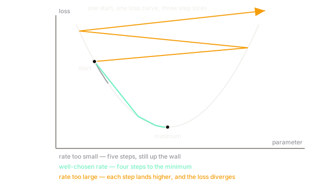
Too large and the loss oscillates or climbs away: each step jumps past the bottom and lands further up the far wall than where it started, so the next step is bigger, and the run walks itself off the edge. Too small and it crawls — the loss falls, flattens somewhere obviously too high, and stalls where the gradient is nearly zero but the loss isn't.

The diagnosis is in the curve's shape, not the final number. Rising from the very first step is the too-large signature. Falling steeply and then flattening far above what the task should allow is the too-small one. Opposite treatments, so read the curve before touching the dial.

What the loop promises, and what it doesn't

On a convex loss — one bowl, no separate dips, see convexity and loss landscapes — a small enough rate provably reaches the global minimum. Linear and logistic regression live there.

A neural network's loss is not convex and gradient descent promises nothing. The textbook picture of that failure is a bowl with side pockets to get stuck in, and in high dimensions it's mostly wrong. A local minimum needs the loss curving upward along every one of millions of directions at once, which is vanishingly unlikely. What you hit instead is saddle points — up some directions, down others — and long flat stretches where progress stops looking like progress. Runs that settle into different minima tend to generalise about as well as each other. The worry is rarely which minimum. It's whether you're still moving.

Show Me the Code

Three rates, one model, three hundred mini-batch steps each. The noise floor is 3600.

1import numpy as np2
3rng = np.random.default_rng(0)4area: np.ndarray = rng.uniform(20.0, 200.0, 2000)          # square metres5rent: np.ndarray = 11.0 * area + 300.0 + rng.normal(0, 60, 2000)6x: np.ndarray = (area - area.mean()) / area.std()          # scale first, or no rate works7
8
9def train(lr: float, batch: int = 256, steps: int = 300) -> float:10    w, b = 0.0, 0.011    for _ in range(steps):12        i = rng.integers(0, x.size, batch)                 # a fresh mini-batch every step13        err = w * x[i] + b - rent[i]14        w -= lr * 2.0 * float((err * x[i]).mean())         # the two partials of the mse15        b -= lr * 2.0 * float(err.mean())16    return float(((w * x + b - rent) ** 2).mean())17
18
19for lr in (0.001, 0.1, 1.02):20    print(f"lr {lr:<6} final mse {train(lr):,.0f}")21    # -> lr 0.001  final mse 785,64522    # -> lr 0.1    final mse 3,58023    # -> lr 1.02   final mse 218,053,181,156,349,088

One factor of ten separates converged from crawling. Another separates crawling from nonsense.

Watch Out For

The Quick Version

• Gradient of the loss with respect to the parameters, step the opposite way by a small multiple of it, repeat.
• Batch: every row, exact, one step per pass. Stochastic: one row, noisy, enormous step counts. Mini-batch of 32 to 512 is what runs.
• The learning rate decides everything, and too large and too small look nothing alike on a loss curve.
• Rising from step one means the rate is too high or the sign is wrong. Falling then flattening too high means it's too low.
• Convex loss plus a small enough rate reaches the global minimum, provably. Neural networks promise nothing.
• In high dimensions the obstacle is saddle points and flat regions, not local minima.

What to Read Next

• Stochastic Gradient Descent argues the noise is doing useful work.
• Momentum fixes the narrow-valley zig-zag no single rate can.
• Adam and AdamW gives every parameter its own effective rate.
• Backpropagation computes the gradient inside a network.
• Loss Functions is what you're descending; the choice reshapes the surface.
• Convexity and Loss Landscapes is where the one-bowl guarantee comes from.
• Definitions worth a look: Gradient, Stationary Point, and Convex Function.