Model-Agnostic Meta-Learning

Why Does This Exist?

Deep neural networks require thousands of labeled examples and millions of gradient descent iterations to learn a new concept. When presented with only 3 to 5 examples of an unseen class (few-shot learning), conventional transfer learning fails: fine-tuning on so few points causes catastrophic overfitting, while frozen feature extractors cannot adapt to out-of-domain distributions.

Prior meta-learning methods engineered specialized memory architectures (such as Neural Turing Machines or recurrent meta-optimizers) or metric spaces (such as Siamese or Prototypical Networks). While effective for narrow classification benchmarks, these methods cannot easily generalize to arbitrary architectures, regression, or reinforcement learning.

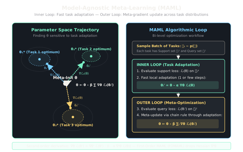
Model-Agnostic Meta-Learning (MAML) treats the optimization process itself as the learning target. By framing meta-learning as bi-level gradient descent, MAML directly finds a set of base parameters $\theta$ that are maximally sensitive to the loss gradients of new tasks, enabling rapid adaptation to unseen problems in just one or two gradient steps without altering the model's architecture.

Think of It Like This

How It Actually Works

Bi-Level Optimization and Second-Order Meta-Gradients

MAML operates across a distribution of tasks $p(\mathcal{T})$. Each task $\mathcal{T}_i$ contains a small support set $\mathcal{D}_i^{\text{train}}$ (e.g., 5 examples for 5-shot learning) and a query set $\mathcal{D}_i^{\text{val}}$ used to measure generalization.

The training procedure consists of an inner loop (task adaptation) nested within an outer loop (meta-optimization):

1. Inner Loop (Task Adaptation): Given base parameters $\theta$ and task $\mathcal{T}_i$, compute the loss on the support set $\mathcal{L}_{\mathcal{T}_i}(\theta, \mathcal{D}_i^{\text{train}})$. Update $\theta$ by one step of gradient descent using inner learning rate $\alpha$:

   $$\theta_i' = \theta - \alpha \nabla_\theta \mathcal{L}_{\mathcal{T}_i}(\theta, \mathcal{D}_i^{\text{train}})$$

2. Outer Loop (Meta-Optimization): Evaluate the adapted parameters $\theta_i'$ on the task's unseen query set $\mathcal{D}_i^{\text{val}}$. The meta-objective sums the query losses across a batch of sampled tasks:

   $$\min_\theta \sum_{\mathcal{T}_i \sim p(\mathcal{T})} \mathcal{L}_{\mathcal{T}_i}(\theta_i', \mathcal{D}_i^{\text{val}})$$

To update the initial parameters $\theta$ using outer learning rate $\beta$, compute the meta-gradient:

Applying the chain rule to expand $\nabla_\theta \mathcal{L}_{\mathcal{T}_i}(\theta_i')$ reveals the second-order derivative:

The term $\nabla_\theta^2 \mathcal{L}_{\mathcal{T}_i}$ is the Hessian matrix of second-order derivatives. While full MAML computes this Hessian-vector product via automatic differentiation, First-Order MAML (FOMAML) approximates $\frac{\partial \theta_i'}{\partial \theta} \approx I$, dropping the Hessian to reduce computational overhead with minimal loss in test accuracy.

Worked Example

Trace a single 1D parameter $\theta$ on two linear regression tasks with inner learning rate $\alpha = 0.1$ and outer learning rate $\beta = 0.2$.

Suppose base weight $\theta = 1.0$.

• Task 1: Target slope is $y = 3x$.

  • Support set: $x_1 = 2$, target $y_1 = 6$.
  • Prediction: $\hat{y}_1 = \theta x_1 = 1.0 \times 2 = 2.0$.
  • Support loss: $\mathcal{L}_1(\theta) = \frac{1}{2}(\hat{y}_1 - y_1)^2 = \frac{1}{2}(2.0 - 6.0)^2 = 8.0$.
  • Support gradient: $\nabla_\theta \mathcal{L}_1 = (\hat{y}_1 - y_1) \cdot x_1 = (-4.0) \times 2 = -8.0$.
  • Inner adaptation: $$\theta_1' = \theta - \alpha (-8.0) = 1.0 - 0.1(-8.0) = 1.8$$
  • Query set: $x_1^{\text{query}} = 1$, target $y_1^{\text{query}} = 3$.
  • Query prediction: $\hat{y}_1^{\text{query}} = \theta_1' \times 1 = 1.8 \times 1 = 1.8$.
  • Query gradient w.r.t $\theta_1'$: $$\nabla_{\theta_1'} \mathcal{L}_1^{\text{query}} = (1.8 - 3.0) \times 1 = -1.2$$

• Task 2: Target slope is $y = -1x$.

  • Support set: $x_2 = 1$, target $y_2 = -1$.
  • Prediction: $\hat{y}_2 = 1.0 \times 1 = 1.0$.
  • Support gradient: $\nabla_\theta \mathcal{L}_2 = (1.0 - (-1.0)) \times 1 = 2.0$.
  • Inner adaptation: $$\theta_2' = \theta - \alpha (2.0) = 1.0 - 0.1(2.0) = 0.8$$
  • Query set: $x_2^{\text{query}} = 2$, target $y_2^{\text{query}} = -2$.
  • Query prediction: $\hat{y}_2^{\text{query}} = 0.8 \times 2 = 1.6$.
  • Query gradient w.r.t $\theta_2'$: $$\nabla_{\theta_2'} \mathcal{L}_2^{\text{query}} = (1.6 - (-2.0)) \times 2 = 3.6 \times 2 = 7.2$$

• Outer Meta-Update (using FOMAML where $\frac{\partial \theta'}{\partial \theta} \approx 1$):

  $$g_{\text{meta}} = \nabla_{\theta_1'} \mathcal{L}_1^{\text{query}} + \nabla_{\theta_2'} \mathcal{L}_2^{\text{query}} = -1.2 + 7.2 = 6.0$$ $$\theta \leftarrow \theta - \beta \cdot g_{\text{meta}} = 1.0 - 0.2(6.0) = 1.0 - 1.2 = -0.2$$

  The base parameter shifts toward negative values to better counter the large error on Task 2.

Code

1import torch2import torch.nn as nn3import torch.optim as optim4from typing import List, Tuple5
6class SimpleMLP(nn.Module):7    def __init__(self) -> None:8        super().__init__()9        self.fc = nn.Linear(1, 1, bias=False)10        self.fc.weight.data.fill_(1.0)11
12    def forward(self, x: torch.Tensor) -> torch.Tensor:13        return self.fc(x)14
15def maml_step(16    model: SimpleMLP,17    tasks: List[Tuple[torch.Tensor, torch.Tensor, torch.Tensor, torch.Tensor]],18    inner_lr: float = 0.1,19    outer_lr: float = 0.220) -> float:21    """Execute one outer meta-update step using higher-order autodiff."""22    meta_loss = 0.023    24    for x_spt, y_spt, x_qry, y_qry in tasks:25        # 1. Inner loop forward & loss on support data26        y_pred = model(x_spt)27        spt_loss = 0.5 * torch.sum((y_pred - y_spt) ** 2)28        29        # 2. Compute inner gradient manually with create_graph=True30        grads = torch.autograd.grad(spt_loss, model.parameters(), create_graph=True)31        32        # 3. Fast adaptation: compute adapted weights theta'33        fast_weights = [w - inner_lr * g for w, g in zip(model.parameters(), grads)]34        35        # 4. Evaluate query loss using adapted weights (functional linear)36        qry_pred = x_qry * fast_weights[0]37        qry_loss = 0.5 * torch.sum((qry_pred - y_qry) ** 2)38        meta_loss = meta_loss + qry_loss39
40    # 5. Outer loop update41    meta_loss_val = meta_loss.item()42    meta_grads = torch.autograd.grad(meta_loss, model.parameters())43    with torch.no_grad():44        for param, grad in zip(model.parameters(), meta_grads):45            param.data -= outer_lr * grad46
47    return meta_loss_val48
49# Task 1: y = 3x, Task 2: y = -x50task1 = (torch.tensor([[2.0]]), torch.tensor([[6.0]]), torch.tensor([[1.0]]), torch.tensor([[3.0]]))51task2 = (torch.tensor([[1.0]]), torch.tensor([[-1.0]]), torch.tensor([[2.0]]), torch.tensor([[-2.0]]))52
53net = SimpleMLP()54loss = maml_step(net, [task1, task2], inner_lr=0.1, outer_lr=0.2)55print(f"Meta loss: {loss:.4f}")56print(f"Updated base weight theta: {net.fc.weight.item():.4f}")57# -> Meta loss: 7.200058# -> Updated base weight theta: -0.0640

Watch Out For

The Quick Version

• Formulates few-shot learning as bi-level optimization over parameter initialization rather than specialized black-box networks.
• Inner loop rapidly updates parameters on small support sets; outer loop updates the base parameters using test query losses.
• Second-order meta-gradients account for how the inner gradient step responds to parameter changes, with first-order approximations providing substantial memory savings.

What to Read Next

• Elastic Weight Consolidation
• Experience Replay Architectures
• Backpropagation