Core ML

Batch Normalization

Standardise each unit's values across the batch, then let the layer learn a scale and shift back. Training uses this batch; inference uses a running average.

One unit's pre-activations sit near 14, where the activation is flat and almost no gradient returns; normalising the batch to mean 0 and spread 1 puts the same values back on the part of the curve that still has slope

Why Does This Exist?

The loss drops for a few hundred steps, then flatlines. Raise the learning rate and it diverges. Lower it and the flatline gets longer. Nothing in the code is wrong.

The model is six layers reading 512×512 satellite tiles and predicting wheat yield. Each layer multiplies its input by weights and sums them — that sum is the pre-activation — then pushes it through a squashing function. The slope of tanh is effectively zero once the input passes about three either way, and a near-zero slope in the activation hands gradient descent a near-zero gradient.

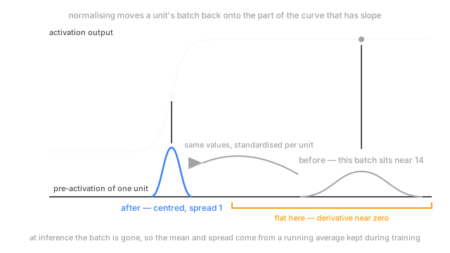
Now the wall. One unit in layer four has pre-activations averaging 14 with a spread of 3, all mapping to 0.9999999 and change. The slope there is 0.00003, so that unit's gradient is three parts in a hundred thousand of what it should be. Alive, contributing nothing. Initialisation put those values near zero at step 0 and stopped mattering by step 500, because the distribution drifts as the layers below it learn.

Think of It Like This

Gain-staging a mixing desk

A compressor only reacts inside a narrow band of levels. Too quiet and it does nothing; too hot and it clamps every peak to the same ceiling.

So the engineer sets a gain knob per channel, one for the kick and one for the vocal, bringing each input to a reference level — not because that level sounds good, but because it's where the next box can hear differences. There's a trim after it, so a vocal that wants to sit hotter goes back up.

Those gains were set at the soundcheck, so you're running numbers measured earlier against a signal arriving now. And a soundcheck of half a second tells you nothing.

How It Actually Works

One mean per unit, taken across the batch

Take one unit and a batch of $m$ examples, collect that unit's $m$ pre-activation values, subtract their mean, divide by their spread, then apply a learned scale and shift.

\hat{z}_i = \frac{z_i - \mu_B}{\sqrt{\sigma_B^2 + \epsilon}}, \qquad y_i = \gamma\,\hat{z}_i + \beta

$z_i$ is that unit's pre-activation for example $i$ . $\mu_B$ and $\sigma_B^2$ are its mean and variance over the batch $B$ — one pair per unit, not per example. $\epsilon$ is a small constant, typically 0.00001, keeping the division safe when a unit is constant across the batch. $\gamma$ and $\beta$ are learned per unit, a scale and a shift, so the layer can undo the normalisation exactly when that's better.

Watch the direction: per feature, across examples. Per unit, or per channel in a convolutional layer, where a channel's statistics pool over every spatial position too. The other cut, per example across features, is layer normalisation, which never touches the batch dimension. That's why transformers use it: sequence models bring variable lengths and small batches, and the per-example version ignores both.

Training and inference compute different functions

During training, $\mu_B$ and $\sigma_B^2$ come from the batch in front of you, so a tile's prediction depends on which other tiles were batched with it. At inference there's no batch, so the layer uses a running average of the training statistics — an exponential moving average, momentum usually 0.9 to 0.99. Same weights, different arithmetic.

Why it helps, and where it fights you

The original paper credited reduced "internal covariate shift": each layer's input distribution stops moving as the layers below it learn. Later work took that apart — inject noise after the normalisation to put the shift back and training still works. The better account is a smoother loss surface, so a larger learning rate stops overshooting, and that rate is where most of the speed-up comes from.

Batch size is where it bites. Those tiles mean 8 fit in memory, and a mean estimated from 8 numbers has a standard error around a third of the spread you're dividing out. The normalisation becomes a noise source — noise in what the layer computes, not jitter in the gradient. Group normalisation is the fix: a group of channels per example, and the batch dimension drops out.

Weight decay on the layer feeding a batch-norm layer also misleads: normalising the output makes the scale of those incoming weights irrelevant, so halving them changes nothing. On ordering — before the activation is the original, and what the formula describes. After works too, a coin flip that matters far less than batch size.

Show Me the Code

One unit drifted to a mean of 14: what normalising does to the surviving gradient, and how far training and eval outputs drift apart.

1import numpy as np2
3
4def bn(z: np.ndarray, mu: np.ndarray, var: np.ndarray, eps: float = 1e-5) -> np.ndarray:5    return (z - mu) / np.sqrt(var + eps)  # one mean and variance per unit, across the batch6
7
8rng = np.random.default_rng(0)9z: np.ndarray = rng.normal(14.0, 3.0, size=(4096, 8))  # pre-activations, drifted off-centre10run_mu, run_var = z.mean(axis=0), z.var(axis=0)  # the running stats inference will use11
12print(f"unnormalised slope {(1.0 - np.tanh(z) ** 2).mean():.5f}")13for n in (256, 8):14    b: np.ndarray = z[:n]15    train: np.ndarray = bn(b, b.mean(axis=0), b.var(axis=0))16    gap: float = float(np.abs(train - bn(b, run_mu, run_var)).mean())17    print(f"batch {n:3d}: slope {(1.0 - np.tanh(train) ** 2).mean():.3f}  train-eval gap {gap:.3f}")18    # -> unnormalised slope 0.0000319    # -> batch 256: slope 0.602  train-eval gap 0.06520    # -> batch   8: slope 0.577  train-eval gap 0.288

Both batch sizes rescue the slope, 0.00003 to about 0.6. The last column matters more: at 256 examples the batch and running statistics differ by 0.065 per value, at 8 by 0.288 — the gap between what training optimised and what inference runs.

Watch Out For

Running statistics that never caught up with the network

Training metrics look healthy and evaluation is bad, sometimes catastrophically. The check is cheap: push one batch through in training mode, then in eval mode, and compare. Diverge wildly and the running averages are your suspect, not the weights.

Two usual causes: too few steps for the moving average to converge — momentum 0.99 needs several hundred steps of a settled distribution — or a final batch-norm layer meeting an evaluation distribution unlike anything in training. Lower the momentum, or freeze the weights and recompute the statistics with a few hundred forward passes.

Batch norm on a batch of eight

Training is unstable, and the same architecture with no normalisation does better. The tell is that raising the batch size fixes it and nothing else does. With 2 to 8 examples the per-batch statistics are noisy enough that the normalisation actively harms training, and on a memory-tight model that batch size isn't negotiable.

Group or layer normalisation is the fix, since both compute statistics per example. One trap: gradient accumulation does not rescue batch norm. It accumulates gradients across micro-batches, but the statistics are still computed inside each one, so the effective batch stays at 8.

The Quick Version

Per feature — each unit or channel — take the mean and variance across the batch, subtract and divide, then apply a learned scale and shift.
Per example across features is layer normalisation instead, which is why transformers pick it.
Training uses this batch's statistics, inference a running average. Two functions, one set of weights.
Small batches and batch norm fight. At 8 examples the statistics are noise, which is why group normalisation exists.
The "internal covariate shift" story doesn't hold up. A smoother loss surface tolerating a larger learning rate is the better account.
Normalising an output makes the scale of the incoming weights irrelevant, so weight decay there isn't what its name suggests.