Core ML

Bayesian Linear Regression

Keep a full distribution over plausible coefficients that narrows as data arrives, so every prediction comes with honest, data-driven uncertainty attached.

A wide, flat prior distribution over the coefficient narrows into a tall, sharp posterior distribution as more data arrives, shifting toward the true value while shedding uncertainty at every step

Why Does This Exist?

Linear regression fit on ten data points and linear regression fit on ten thousand data points both return one coefficient per feature — a single number, with nothing in the output distinguishing "this number is well-supported" from "this number is a rough guess from very little evidence." A hospital using a regression model to estimate treatment effect from a small pilot study genuinely needs to know the difference: a coefficient of 2.0 from ten patients and a coefficient of 2.0 from ten thousand patients should not be treated with equal confidence, and ordinary linear regression's output gives no way to tell them apart.

Bayesian linear regression answers this directly by treating each coefficient not as a single number to solve for, but as a probability distribution to update. Start with a prior distribution reflecting what's plausible before seeing any data, and update it into a posterior distribution using Bayes' theorem once data arrives — a posterior that's naturally wide when evidence is thin and naturally narrow when evidence is abundant.

Think of It Like This

A jury's confidence sharpening as testimony accumulates

A jury walks into a trial with only a rough sense of what might have happened — a wide range of plausible stories, none ruled out. As witnesses testify and evidence is presented, that wide range narrows: some stories become implausible, others gain support, and the jury's collective belief sharpens around a smaller set of possibilities.

After one witness, the jury's belief is still broad — reasonable people could still disagree. After a dozen consistent witnesses, that same belief has narrowed dramatically around one account. The jury never had a single "the answer is X" moment; what narrowed over time was the whole distribution of what they considered plausible. Bayesian linear regression tracks exactly that kind of narrowing, formally, for a model's coefficients.

How It Actually Works

Prior, likelihood, posterior

Before seeing any data, a prior distribution over each coefficient $w$ encodes what's considered plausible — commonly a normal distribution centered at zero, expressing mild belief that most coefficients are probably small unless the data says otherwise. Given training data, the likelihood measures how well any particular value of $w$ would have explained the observed outcomes. Bayes' theorem combines the two into the posterior:

p(w \mid \text{data}) \propto p(\text{data} \mid w) \, p(w)

The posterior is itself a full distribution over $w$ , not a single value — it's simultaneously a statement of the most plausible coefficient value and a statement of how confident that value actually is.

Why the posterior narrows with more data

With a normal prior and normal noise — the standard setup — the posterior over $w$ is also exactly normal, and its variance shrinks as more data arrives, since each new observation contributes additional evidence pinning the coefficient down further. This isn't an approximation; for this particular combination of prior and likelihood, called a conjugate prior, the update has an exact closed form, and the posterior's shrinking spread is a direct, provable consequence of accumulating evidence rather than a heuristic.

MAP estimation: the bridge back to ordinary regression

Taking the single most probable value from the posterior — its peak — is called maximum a posteriori (MAP) estimation, and it connects this page directly to already-familiar territory: MAP estimation with a normal prior on the coefficients produces exactly the same point estimate as ridge regression. Ridge's L2 penalty isn't an arbitrary add-on; it's what a normal prior on the coefficients looks like once you throw away everything except the posterior's peak. Bayesian linear regression keeps the whole distribution instead of collapsing it to that one point, which is precisely what buys back the uncertainty ridge regression discards.

Predictive uncertainty, not just coefficient uncertainty

Because the coefficients themselves are a distribution, a prediction for a new input isn't one number either — it's a distribution over plausible outcomes, wider where the model has seen less relevant data and narrower where it's well-supported. This predictive distribution is what a Bayesian approach hands back that a point-estimate approach fundamentally cannot: not just "the prediction is 2.0" but "the prediction is 2.0, and here's the honest range of other values still plausible given what's been observed."

Show Me the Code

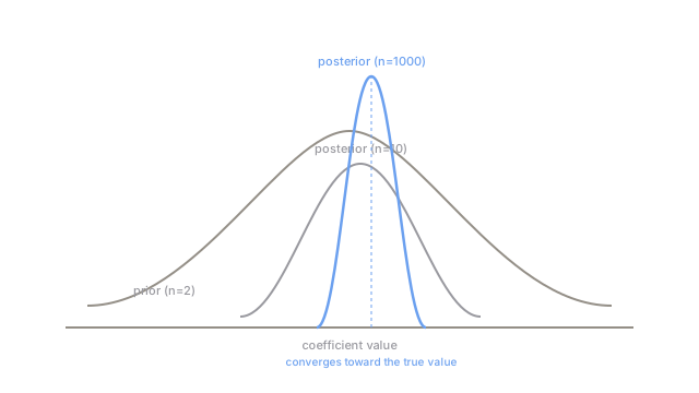
Updating a coefficient's posterior distribution as sample size grows, watching it narrow and converge toward the true value.

1import numpy as np2
3
4def bayes_update(x: np.ndarray, y: np.ndarray, prior_mean: float, prior_var: float, sigma: float) -> tuple[float, float]:5    """Posterior for w in y = w*x + noise, noise ~ N(0, sigma^2), given a normal prior."""6    precision_prior = 1 / prior_var7    precision_data = np.sum(x ** 2) / sigma ** 28    post_var = 1 / (precision_prior + precision_data)9    post_mean = post_var * (prior_mean * precision_prior + np.sum(x * y) / sigma ** 2)10    return post_mean, post_var11
12
13rng = np.random.default_rng(2)14true_w, sigma_noise = 2.0, 1.015prior_mean, prior_var = 0.0, 10.0  # weak, wide prior16for n in (2, 10, 100, 1000):17    x = rng.normal(0, 1, n)18    y = true_w * x + rng.normal(0, sigma_noise, n)19    post_mean, post_var = bayes_update(x, y, prior_mean, prior_var, sigma_noise)20    print(f"n={n:4d}: posterior mean = {post_mean:.3f}, posterior std = {np.sqrt(post_var):.4f}")21# -> n=   2: posterior mean = 4.441, posterior std = 1.563622# -> n=  10: posterior mean = 2.095, posterior std = 0.364523# -> n= 100: posterior mean = 2.051, posterior std = 0.099524# -> n=1000: posterior mean = 1.986, posterior std = 0.0312

At $n=2$ , the posterior is both far from the true value of 2.0 and admits it — a standard deviation over 1.5 wide. By $n=1000$ , the posterior mean sits almost exactly on the true value, and its standard deviation has shrunk roughly 50-fold. The number itself gets better, and critically, the model's stated confidence in that number tracks how much evidence actually supports it.

Watch Out For

Reporting the MAP point estimate and discarding the posterior width

Taking only the posterior's peak throws away exactly the information this method exists to provide, and produces a result numerically identical to ridge regression — at which point the extra machinery bought nothing. If uncertainty isn't going to be used downstream, ordinary or ridge regression is simpler and equivalent; use the full Bayesian treatment specifically when the predictive uncertainty itself is needed.

Choosing a strong, informative prior without stating the assumption

A prior with a small variance can dominate the posterior when data is scarce, effectively deciding the answer before the data gets much say — and this can happen quietly, without anyone examining the prior's actual influence. Check how much the posterior would change if the prior were weakened, especially in small-sample settings, and state the chosen prior's assumptions explicitly rather than letting a default setting make the decision implicitly.

The Quick Version

Bayesian linear regression treats coefficients as probability distributions, updated from a prior into a posterior using Bayes' theorem as data arrives.
With a normal prior and normal noise, the posterior is exactly normal too, and its variance provably shrinks as more data accumulates.
Taking the posterior's peak (MAP estimation) with a normal prior produces the same point estimate as ridge regression — ridge's L2 penalty is a normal prior in disguise.
The real payoff is predictive uncertainty: a full distribution over plausible outcomes for a new input, not just a single best-guess number.