Core ML

Bayesian Optimization

A surrogate model predicts both a score and its uncertainty everywhere, and an acquisition function picks the next expensive trial from that belief map.

A surrogate curve fitted to three past trials is tight where they were measured and wide everywhere else, and the acquisition function peaks at a point that is both promising and still genuinely uncertain

Why Does This Exist?

Hyperparameter tuning covers the menu — grid, random, successive halving — and ends on the case where none of them are good enough: training itself is slow, so every evaluation is expensive, and choosing badly wastes hours instead of milliseconds.

Here's the case we'll carry down the page. You're tuning the learning rate for a model that takes forty minutes to train per run, and your budget is maybe fifteen runs before the deadline. Random search treats every run as unrelated to the last, drawing each learning rate independently no matter what the previous fourteen just told you. After run three, you already know the score falls off sharply below a certain rate and plateaus above another — a human tuning by hand would use that. Random search can't, by construction: it has no memory of what it already learned.

Bayesian optimization is what remembering does for this problem, made precise enough to automate.

Think of It Like This

Prospecting for oil with one drill and a map that updates itself

You're deciding where to drill for oil across a large field, and each borehole costs a fortune, so you get maybe a dozen. After each hole you don't just log a number — you update a belief about the whole field: nearby ground probably resembles what you just found, and ground you haven't drilled near at all could be anything.

Drilling only where past holes struck oil ignores the vast unexplored ground that might be even richer. Drilling only where you're most uncertain wastes fortunes confirming that empty ground is, in fact, empty. The prospector who wins balances both: drill somewhere that's either promising or genuinely unknown, never somewhere both mediocre and already understood.

That belief-updating map is the surrogate model. The balancing rule for where to drill next is the acquisition function.

How It Actually Works

The surrogate: a cheap stand-in for an expensive function

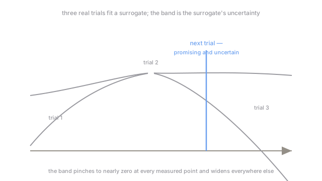
You want to know how a hyperparameter setting scores on validation, but evaluating it means a full training run. A surrogate model — almost always a Gaussian process — is fitted instead to every (setting, score) pair measured so far, and it's cheap to query anywhere, including settings you've never actually tried. Crucially, a Gaussian process hands back both a predicted score and an uncertainty at every point, tight near settings you've measured and wide everywhere else — exactly the map the prospector is updating.

The acquisition function: turning a belief into the next move

The surrogate alone doesn't say where to look next; an acquisition function turns its predictions and uncertainties into a single number ranking every candidate setting, and the next real evaluation goes wherever that number peaks. Expected improvement, the most common choice, scores a point high when the surrogate predicts a good result, high uncertainty, or both — so a point that might plausibly beat the best score seen so far, even if the surrogate isn't sure, can still win. That's the exploration/exploitation balance: pure exploitation always drills next to the last strike and gets stuck on a local optimum; pure exploration wanders the whole field and never closes in.

Why this earns its keep only when evaluations are expensive

Fitting the Gaussian process and maximising the acquisition function cost real compute — nowhere near a full training run, but not free either. Random search wastes evaluations on points that turn out uninformative; Bayesian optimization spends that same overhead choosing better points instead. The trade only pays when a real evaluation dwarfs the surrogate's cost, which is exactly the forty-minutes-a-run setting this page opened with. For a model that trains in half a second, the overhead of fitting a Gaussian process on every step outweighs anything the smarter choice buys you, and plain random search wins on wall-clock time.

Show Me the Code

Three runs logged already; fit the surrogate, score expected improvement across the range, and see where it sends the next trial.

1import numpy as np2
3rng = np.random.default_rng(2)4
5def true_score(lr: np.ndarray) -> np.ndarray:  # the real, expensive-to-evaluate validation score6    return -12.0 * (np.log10(lr) + 2.0) ** 2 + 5.07
8def rbf(a: np.ndarray, b: np.ndarray, length: float = 0.6) -> np.ndarray:9    return np.exp(-((a[:, None] - b[None, :]) ** 2) / (2 * length ** 2))10
11tried = np.log10(np.array([1e-4, 1e-1, 1.0]))          # three runs spent so far12scores = true_score(10 ** tried)13grid = np.linspace(-4, 0, 200)14
15K = rbf(tried, tried) + 1e-6 * np.eye(3)16K_star = rbf(grid, tried)17mean = K_star @ np.linalg.solve(K, scores)18var = 1.0 - np.sum(K_star @ np.linalg.inv(K) * K_star, axis=1)19
20best_so_far = scores.max()21z = (mean - best_so_far) / np.sqrt(np.maximum(var, 1e-12))22expected_improvement = np.sqrt(var) * (z * 0.5 * (1 + np.tanh(z)) + np.exp(-z ** 2 / 2) / np.sqrt(2 * np.pi))23next_lr = 10 ** grid[np.argmax(expected_improvement)]24
25print(f"three runs so far, best score {best_so_far:.2f} at lr={10**tried[np.argmax(scores)]:.4f}")26print(f"surrogate's most promising unexplored point -> try lr={next_lr:.4f} next")27print(f"true score there: {true_score(np.array([next_lr]))[0]:.2f}")28# -> three runs so far, best score -7.00 at lr=0.100029# -> surrogate's most promising unexplored point -> try lr=0.0215 next30# -> true score there: 3.68

The best of the three manual-looking runs scored -7.00. Expected improvement points at a learning rate none of the three tries came close to, purely from the shape of the uncertainty between them, and it scores 3.68 there — a fourth run that beats all three predecessors combined.

Watch Out For

Using Bayesian optimization on a search that's cheap to evaluate

Fitting a Gaussian process and maximising an acquisition function costs real wall-clock time on every iteration, and for a model that trains in seconds, that overhead can exceed the cost of just running a hundred random configurations directly. Check the ratio of one real evaluation's cost to the surrogate's own fitting cost before reaching for this; below a few seconds per evaluation, random search plus successive halving is usually faster in total wall-clock time despite trying more configurations.

Trusting the surrogate in a region with almost no real evaluations nearby

A Gaussian process reports high uncertainty far from any data it has seen, which is honest — but a badly chosen kernel or too few initial points can also make it confidently wrong in a sparse region, especially early in a search when only two or three points exist. Seed the search with a handful of points spread across the whole range before letting the acquisition function take over, so the surrogate has enough real signal to make its own uncertainty estimate meaningful rather than an artifact of the kernel's prior.

The Quick Version

A surrogate model, usually a Gaussian process, is fitted to every (hyperparameter, score) pair measured so far and predicts both a value and an uncertainty anywhere, including unseen settings.
An acquisition function, most commonly expected improvement, turns those predictions into a single ranking of where to evaluate next, balancing a good predicted score against high uncertainty.
The method only earns its overhead back when a real evaluation is expensive — a slow training run — compared to fitting the surrogate itself.
Seed the search with a handful of spread-out points before trusting the acquisition function; a surrogate fitted on two or three points can be confidently wrong.
For fast-to-evaluate settings, plain random search or successive halving usually wins on total wall-clock time.