Core ML

Gaussian Process Regression

Put a prior directly over the space of possible functions, rather than a fixed set of coefficients, and let the data narrow it to the ones that fit.

A mean prediction curve runs through three known training points with almost no uncertainty band around it there, and the uncertainty band widens visibly in the gaps between points and especially far from all of them

Why Does This Exist?

Bayesian linear regression keeps a distribution over coefficients rather than one fixed answer, and that solves the uncertainty problem for anything shaped like a straight line — or, with polynomial features, anything shaped like a fixed-degree curve. It still has to commit to a functional form in advance: pick the degree, pick the features, and the shape of the answer is locked in before any data arrives.

A Gaussian process sidesteps choosing a functional form at all. Instead of a prior over a fixed set of coefficients, it places a prior directly over the space of all possible functions that could explain the data — infinitely more flexible than committing to a polynomial degree — and lets the data narrow that space down to whichever functions actually pass through, or near, the points observed. The price, made explicit below, is a computational cost that grows fast with data size.

Think of It Like This

Threading string through fixed pegs on a board

Imagine every possible smooth curve as a piece of elastic string laid across a board, and a Gaussian process's prior is "any of these strings is plausible, some more likely than others depending on how wiggly they are." Now hammer in a few pegs at exact known points — the training data — and every string that doesn't pass through those pegs gets discarded. What's left is a bundle of strings that all agree closely near the pegs and fan out into a spread of possibilities everywhere a peg hasn't pinned them down.

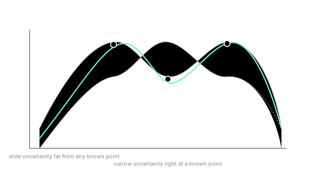
That fan of remaining strings, tight near data and wide everywhere else, is exactly a Gaussian process's predictive distribution — not one curve, but a whole plausible bundle, with its spread telling you directly where the pegs actually constrained the answer and where they didn't.

How It Actually Works

The kernel is the modeling assumption

A Gaussian process is defined entirely by a kernel function $k(x, x')$ , which measures how correlated two points' function values are expected to be, purely based on their inputs. The most common choice, the RBF (radial basis function) kernel,

k(x, x') = \exp\left(-\frac{(x - x')^2}{2\ell^2}\right)

says nearby $x$ values should have highly correlated outputs, with correlation falling off smoothly as distance grows, governed by the length scale $\ell$ . This kernel is the model — choosing it is the entire modeling decision, replacing the choice of polynomial degree or feature set in earlier methods. Different kernels encode different assumptions: periodic kernels for cyclical data, kernels with different smoothness for rougher or smoother underlying functions.

Prediction as conditioning a joint distribution

A Gaussian process treats the function values at any finite set of points as jointly normally distributed, with covariances given directly by the kernel. Predicting at new points is then pure probability: condition that joint normal distribution on the known training values, and standard multivariate-normal algebra hands back both a mean prediction and a full covariance — no gradient descent, no optimization loop, at prediction time.

\mu_* = K_* K^{-1} y, \qquad \Sigma_* = K_{**} - K_* K^{-1} K_*^\top

$K$ is the kernel matrix between training points, $K_*$ between new points and training points, $K_{**}$ between new points and themselves, and $y$ the training outputs. $\mu_*$ is the predictive mean; the diagonal of $\Sigma_*$ gives the predictive variance — directly and automatically wide wherever training data is sparse, exactly the mechanism the diagram shows.

The uncertainty comes free, and the cost is real

Because the whole prediction is a single conditioning operation on a joint distribution, uncertainty isn't an add-on computed separately — it falls straight out of the same matrix algebra that produces the mean. That's the "comes free" half of this page's framing. The other half is the $K^{-1}$ term: inverting an $n \times n$ kernel matrix costs $O(n^3)$ time, which is entirely tractable at a few hundred points and becomes prohibitive well before a few tens of thousands. This cubic wall is the specific, well-known reason Gaussian processes dominate small-data, high-value settings — Bayesian optimization's surrogate models, scientific experiment design — and essentially never appear as a direct model for large-scale data.

Show Me the Code

Predicting at five query points from three known points, and watching predictive uncertainty shrink at known points and grow far from them.

1import numpy as np2
3
4def rbf_kernel(x1: np.ndarray, x2: np.ndarray, length_scale: float = 1.0) -> np.ndarray:5    dists = (x1[:, None] - x2[None, :]) ** 26    return np.exp(-dists / (2 * length_scale ** 2))7
8
9x_train = np.array([-2.0, 0.0, 2.0])10y_train = np.array([0.5, -1.0, 0.8])11x_query = np.array([-2.0, -1.0, 0.0, 1.0, 4.0])  # 4.0 is far from any training point12
13K = rbf_kernel(x_train, x_train) + 1e-6 * np.eye(3)  # small jitter for numerical stability14K_star = rbf_kernel(x_query, x_train)15K_star_star = rbf_kernel(x_query, x_query)16K_inv = np.linalg.inv(K)17
18posterior_mean = K_star @ K_inv @ y_train19posterior_var = np.diag(K_star_star - K_star @ K_inv @ K_star.T)20for xq, mean, var in zip(x_query, posterior_mean, np.sqrt(posterior_var)):21    print(f"x={xq:5.1f}: mean={mean:+.3f}  std={var:.4f}")22# -> x= -2.0: mean=+0.500  std=0.001023# -> x= -1.0: mean=-0.326  std=0.590024# -> x=  0.0: mean=-1.000  std=0.001025# -> x=  1.0: mean=-0.148  std=0.590026# -> x=  4.0: mean=+0.130  std=0.9906

At $x=-2.0$ and $x=0.0$ — both exact training points — the standard deviation collapses to almost zero, since the model is certain about points it's directly observed. At $x=4.0$ , far outside the training range entirely, the standard deviation climbs to 0.99, close to the prior's own uncertainty — the model is honestly admitting it has learned almost nothing about that region.

Watch Out For

Applying a Gaussian process to a dataset with tens of thousands of points

The $O(n^3)$ inversion cost makes a direct Gaussian process impractical well before large-scale territory — a few thousand points is often already the edge of comfortable, and tens of thousands is generally out of reach without specialized sparse or approximate methods. Check the intended data size before reaching for a plain Gaussian process, and look into inducing-point or sparse approximations if the data volume is genuinely large.

Trusting predictions extrapolated on a poorly chosen kernel

The kernel encodes strong assumptions about smoothness and correlation structure, and a mismatched kernel — assuming smoothness the real function doesn't have, or the wrong length scale — produces confident-looking predictions and uncertainty bands that don't reflect the model's real ignorance. Kernel choice and its hyperparameters (like length scale) deserve as much scrutiny as any other model's architecture choice, not a default left unexamined.

The Quick Version

A Gaussian process places a prior directly over functions, defined entirely by a kernel measuring how correlated two points' outputs should be.
Prediction is conditioning a joint normal distribution on known data — pure probability algebra, with no separate optimization step.
Predictive uncertainty comes directly from that same conditioning operation, automatically wide where data is sparse and narrow near observed points.
The kernel-matrix inversion costs $O(n^3)$ , which is the specific, well-known reason Gaussian processes stay confined to small or medium-sized datasets.