Core ML

Hyperparameter Tuning

Grid search spends its budget evenly across knobs whether or not they matter. Random search spends that same budget where the score actually responds.

With the same evaluation budget, a grid spends five distinct values on the knob that matters while random search draws far more, because each of its points is independent rather than fixed to a lattice

Why Does This Exist?

Every model in this band has knobs that training doesn't set for you: how deep a tree grows, how many neighbours a KNN model votes, how much a ridge penalty shrinks. Get one wrong by an order of magnitude and a good algorithm loses to a mediocre one tuned properly.

Here's the case we'll carry down the page. You're tuning a gradient-boosted tree for a churn model: learning rate, max depth, and number of leaves, three knobs whose good values depend on each other in ways no formula gives you in advance. A validation set exists to score any one setting honestly. What it doesn't tell you is which setting to try next, and with three knobs and even a modest range each, the space of combinations is already in the thousands.

That search — which combinations to actually run, out of everything you could — is what hyperparameter tuning names.

Think of It Like This

Tasting a soup you can only adjust one spoonful at a time

You're seasoning a large pot of soup, and you're only allowed to taste one spoonful — one combination of salt, acid, and heat — before deciding on your next attempt. Salt matters enormously; the amount of black pepper you add barely changes the taste at all, but you don't know that going in.

Grid search means you decided beforehand, on paper, to try every combination of five salt levels and five pepper levels laid out on an even lattice, whether or not the tasting so far told you pepper was a waste of spoonfuls. Random search throws both amounts independently each time, so across the same number of tastings, salt still gets tried at many different levels even though pepper — the one that didn't matter — ate a fifth of the grid's attempts for nothing. Bayesian optimization is the cook who remembers every taste so far and chooses the next spoonful specifically to resolve whichever uncertainty seems most likely to matter.

How It Actually Works

Grid search tries every combination, and pays for dimensions that don't matter

Grid search lays out a fixed set of values per hyperparameter and evaluates every combination — five learning rates by five depths is 25 runs, and a third knob turns that into 125. It's simple, exhaustive over the grid you chose, and its cost multiplies with every dimension you add, which stops being affordable past three or four knobs.

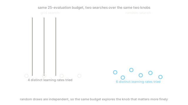
The deeper problem, formalised by Bergstra and Bengio in 2012, is that a grid spends its budget evenly across dimensions regardless of which ones matter. If depth barely moves your score and learning rate is everything, a 5-by-5 grid still only tries 5 distinct learning-rate values — the other 20 evaluations bought you finer resolution on a knob that didn't need it.

Random search spends the same budget where it actually helps

Random search draws each hyperparameter independently from its range, for the same total number of evaluations. Because every draw is independent, a budget of 25 tries 25 distinct values of learning rate, not 5 — so the dimension that matters gets explored at the resolution a grid would only afford if you'd known in advance to allocate it there.

Bayesian optimization spends the budget where the model of the search says to look

Both grid and random search choose every point in advance, blind to what earlier evaluations found. Bayesian optimization fits a surrogate model — commonly a Gaussian process — to the (hyperparameters, validation score) pairs measured so far, then picks the next point by balancing exploring where the surrogate is most uncertain against exploiting where it predicts the score is highest. Each real evaluation is expensive — a full training run — so spending a little compute on the surrogate to choose better is a good trade once training itself is slow.

Successive halving throws away bad candidates early, cheaply

A different lever entirely: instead of choosing hyperparameters more cleverly, spend less on the candidates that are clearly losing. Successive halving starts many candidates on a small budget — a few epochs, a data subsample — keeps the best fraction, doubles their budget, and repeats. A candidate that's clearly bad after one epoch rarely becomes the best after a hundred, so most of the compute concentrates on the candidates worth the full budget. Random search plus successive halving, run together, is a strong practical default before reaching for a full Bayesian search.

Show Me the Code

Same 25-evaluation budget, two knobs, one that matters and one that doesn't. Grid search spends five distinct values on the one that matters; random search spends far more.

1import numpy as np2
3rng = np.random.default_rng(9)4best_log_lr = -1.5  # optimum sits at lr ~ 0.0316, deliberately off the grid's nodes5
6def val_score(log_lr: float, depth: float) -> float:7    # only log(lr) matters; depth is a red herring the grid still spends budget on8    return -(log_lr - best_log_lr) ** 2 - 0.001 * (depth - 5) ** 29
10lr_grid = np.linspace(-4, 0, 5)      # 5 log-lr values ...11depth_grid = np.linspace(1, 9, 5)    # ... x 5 depth values = 25 evaluations12grid_best = max(val_score(lr, d) for lr in lr_grid for d in depth_grid)13
14log_lr_rand = rng.uniform(-4, 0, 25)  # 25 draws, each an independent (lr, depth) pair15depth_rand = rng.uniform(1, 9, 25)16rand_best = max(val_score(lr, d) for lr, d in zip(log_lr_rand, depth_rand))17
18closest_grid_lr = min(abs(v - best_log_lr) for v in lr_grid)19closest_rand_lr = min(abs(v - best_log_lr) for v in log_lr_rand)20print(f"closest log10(lr) to the true optimum: grid={closest_grid_lr:.3f}  random={closest_rand_lr:.3f}")21print(f"best validation score reached:         grid={grid_best:.4f}  random={rand_best:.4f}")22# -> closest log10(lr) to the true optimum: grid=0.500  random=0.08723# -> best validation score reached:         grid=-0.2500  random=-0.0078

Both searches spent 25 evaluations. Random search lands more than five times closer to the true optimum, because it never wasted resolution on the depth axis, which the score barely responded to.

Watch Out For

Tuning hyperparameters against the test set

The symptom shows up months later: a model that scored well in development quietly underperforms in production, by a margin the original numbers never warned about. It happens whenever the test set gets checked repeatedly while choosing hyperparameters — each check is a small peek, and forty small peeks add up to the test set becoming a second training set. Tune only against a validation set or cross-validation folds, and touch the test set exactly once, after every hyperparameter decision is final.

Searching a range that was never wide enough to contain the answer

A search that returns its best result sitting at the edge of the range you specified — the largest learning rate allowed, the deepest tree — is reporting that your range was too narrow, not that it found an answer. Check the winning values against the search space's boundaries before trusting the result, and widen the range and rerun rather than shipping an edge case as an optimum.

The Quick Version

Grid search evaluates every combination on a fixed lattice, and its cost multiplies with every hyperparameter you add.
Random search draws each hyperparameter independently, so a fixed budget still explores the dimension that matters at high resolution, even without knowing in advance which dimension that is.
Bayesian optimization fits a surrogate model to the evaluations run so far and chooses the next point to balance exploring uncertainty against exploiting a predicted good score — worth it once each real evaluation is expensive.
Successive halving cuts cost a different way: run many candidates cheaply, keep the best fraction, and give only survivors a full budget.
Random search plus successive halving is a strong, cheap default. Reach for Bayesian optimization when each full training run is slow enough that choosing points well is worth the extra overhead.
A result sitting at the edge of your search range is a sign the range was wrong, not that the search found an answer.