Circuit Discovery Methodologies

By surgically swapping intermediate activations between clean and corrupted prompts, circuit discovery isolates the exact sub-network of attention heads and neurons causally responsible for a model's prediction.

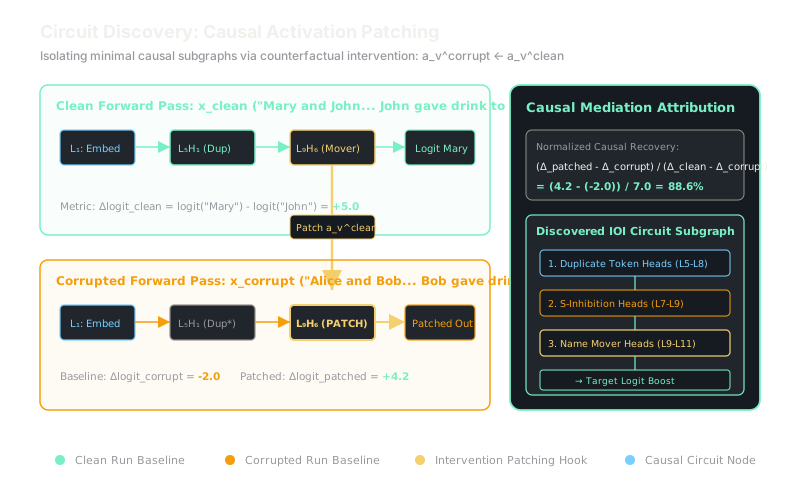
Activation patching workflow: swapping intermediate activations between clean and corrupted runs to isolate causal circuit edges.

Why Does This Exist?

A 70-billion parameter Large Language Model executes trillions of floating-point operations for every single generated token. When the model correctly answers a grammar puzzle, tracks a variable across Python code, or executes Indirect Object Identification (e.g., "When Mary and John went to the store, John gave a drink to [Mary]"), looking at the full network is overwhelming. Millions of parameters are firing simultaneously.

However, empirical research by Wang et al. and the mechanistic interpretability community revealed that individual tasks do not require the whole model. Instead, specific reasoning behaviors are computed by a tiny, sparse sub-graph of nodes—often fewer than 30 attention heads and MLP layers out of thousands. The remaining 99.9% of the network acts as an identity pass-through for that task.

Traditional correlational methods (such as attention weights or probing classifiers) fail to find this sub-graph because correlated activations are not necessarily causal. A head might attend strongly to "Mary" simply because it echoes proper nouns everywhere, without transmitting that information to the final output logits. Circuit discovery methodologies provide rigorous causal interventional frameworks—such as activation patching, causal tracing, and Edge Attribution Patching (EAP)—to surgically isolate, verify, and document the minimal causal circuits responsible for specific model capabilities.

Think of It Like This

Swapping circuit board chips between working and broken radios

Imagine you possess two identical vintage radios: Radio A and Radio B. Radio A plays clean, crisp FM music. Radio B only outputs loud, staticky white noise.

You want to find which component on the circuit board is responsible for tuning the FM frequency. You do not probe every wire with an oscilloscope and guess from electrical hums.

Instead, you use an interventional chip-swapping protocol. While both radios are plugged into power, you take Chip #1 from Radio A and swap it into Radio B. If Radio B still produces static, Chip #1 is irrelevant. You repeat this across the board. Suddenly, when you transplant Chip #7 from Radio A into Radio B, Radio B's static vanishes and it instantly plays clear music.

By performing a controlled surgical transplant, you have proven with causal certainty that Chip #7 is the frequency demodulator, regardless of what the other 50 chips on the board are doing.

How It Actually Works

Activation Patching and Causal Mediation Metrics

Circuit discovery converts qualitative hypotheses into quantifiable causal experiments through activation patching (also known as interchange intervention or causal mediation analysis):

1. Define Contrastive Pairs

Create a clean prompt $x_{\text{clean}}$ and a corrupted counterpart $x_{\text{corrupt}}$ that differs only by the target entity:

$x_{\text{clean}}$ : "When Mary and John went to the store, John gave a drink to" $\to$ Target: Mary
$x_{\text{corrupt}}$ : "When Alice and Bob went to the store, Bob gave a drink to" $\to$ Target: Alice

We define the primary performance metric as the difference between the target logit and the distractor logit at the final token position:

\Delta \text{logit}(x) = \text{logit}(\text{Target}) - \text{logit}(\text{Distractor})

2. Run Forward Baselines

Run both prompts through the network without intervention and record internal activation caches:

$\Delta \text{logit}_{\text{clean}} = \text{logit}_{\text{clean}}(\text{Mary}) - \text{logit}_{\text{clean}}(\text{John}) > 0$ (High positive score)
$\Delta \text{logit}_{\text{corrupt}} = \text{logit}_{\text{corrupt}}(\text{Mary}) - \text{logit}_{\text{corrupt}}(\text{John}) \le 0$ (Negative or zero score)

3. Perform Activation Patching Interventions

To test whether node $v$ (an attention head or MLP layer at layer $l$ ) is causally responsible for transmitting the correct entity:

Pass $x_{\text{corrupt}}$ through the model.
At layer $l$ , hook node $v$ 's output and overwrite it with the cached activation from the clean run:

a_v^{\text{patched}} \leftarrow a_v^{\text{clean}}

Allow all subsequent layers to execute normally using the patched activation.
Measure the patched logit difference $\Delta \text{logit}_{\text{patched}}$ .

4. Compute Normalized Causal Mediation Effect

We normalize the recovery score to measure what fraction of the clean behavior was restored solely by restoring node $v$ :

\text{Normalized Effect}(v) = \frac{\Delta \text{logit}_{\text{patched}} - \Delta \text{logit}_{\text{corrupt}}}{\Delta \text{logit}_{\text{clean}} - \Delta \text{logit}_{\text{corrupt}}}

$\text{Effect} \approx 1.0$ : Node $v$ is a primary causal bottleneck carrying the essential information.
$\text{Effect} \approx 0.0$ : Node $v$ is functionally inert for this task.

5. Scaled Circuit Discovery via Edge Attribution Patching (EAP)

Iterating activation patching over every individual edge in a network requires $\mathcal{O}(E)$ forward passes, taking days of GPU compute. Modern discovery pipelines use Edge Attribution Patching (EAP), which linearizes the intervention using a single backward pass gradient:

\text{Attribution}(u \to v) \approx \left( a_u^{\text{clean}} - a_u^{\text{corrupt}} \right) \cdot \nabla_{a_u} \mathcal{L}_{\text{corrupt}}

EAP evaluates all candidate edges across a 30-layer model in seconds, pruning the graph to leave only the verified minimal circuit.

Worked Example

Let us evaluate the causal importance of two candidate attention heads in a 12-layer language model executing the Indirect Object Identification (IOI) task.

Clean run logit difference: $\text{logit}(\text{Mary}) = 8.5$ , $\text{logit}(\text{John}) = 3.5 \implies \Delta \text{logit}_{\text{clean}} = 8.5 - 3.5 = +5.0$
Corrupted run logit difference: $\text{logit}(\text{Mary}) = 2.0$ , $\text{logit}(\text{John}) = 4.0 \implies \Delta \text{logit}_{\text{corrupt}} = 2.0 - 4.0 = -2.0$
Denominator (total task swing): $\Delta \text{logit}_{\text{clean}} - \Delta \text{logit}_{\text{corrupt}} = 5.0 - (-2.0) = 7.0$

Test Candidate A: Attention Head Layer 9, Head 6 (L9H6) We execute the corrupted prompt, but freeze and patch the output of L9H6 with its clean activation:

Patched output logits: $\text{logit}(\text{Mary}) = 6.2$ , $\text{logit}(\text{John}) = 2.0 \implies \Delta \text{logit}_{\text{patched}} = 6.2 - 2.0 = +4.2$
Compute Normalized Causal Effect:

\text{Normalized Effect}(\text{L9H6}) = \frac{4.2 - (-2.0)}{7.0} = \frac{6.2}{7.0} \approx 0.8857 \quad (88.6\%)

Transplanting this single attention head alone restores 88.6% of the model's clean capability. L9H6 is verified as a primary Name Mover Head.

Test Candidate B: Attention Head Layer 4, Head 1 (L4H1) We repeat the experiment, patching L4H1 instead:

Patched output logits: $\text{logit}(\text{Mary}) = 2.1$ , $\text{logit}(\text{John}) = 3.9 \implies \Delta \text{logit}_{\text{patched}} = 2.1 - 3.9 = -1.8$
Compute Normalized Causal Effect:

\text{Normalized Effect}(\text{L4H1}) = \frac{-1.8 - (-2.0)}{7.0} = \frac{0.2}{7.0} \approx 0.0286 \quad (2.9\%)

Transplanting L4H1 only recovers 2.9% of the metric. L4H1 is causally pruned from the circuit.

Code

Below is a self-contained Python implementation demonstrating an activation patching harness on a toy computation graph:

1import numpy as np2
3
4class ToyTransformerNode:5    """Simulates a modular attention head or MLP layer."""6
7    def __init__(self, weight: float, bias: float) -> None:8        self.weight = weight9        self.bias = bias10
11    def forward(self, x: float) -> float:12        return self.weight * x + self.bias13
14
15class ToyGraphModel:16    """Toy 3-stage model: Input -> [Node A, Node B] -> Final Logit Head."""17
18    def __init__(self) -> None:19        self.node_a = ToyTransformerNode(weight=1.8, bias=0.2)  # Causal carrier20        self.node_b = ToyTransformerNode(weight=0.1, bias=0.0)  # Distractor node21
22    def run(self, x: float, patch_a: float | None = None, patch_b: float | None = None) -> tuple[float, float, float]:23        act_a = self.node_a.forward(x)24        act_b = self.node_b.forward(x)25
26        # Apply surgical interventional patches if present27        if patch_a is not None:28            act_a = patch_a29        if patch_b is not None:30            act_b = patch_b31
32        # Final readout layer combining activations33        output_logit = 2.0 * act_a + 0.5 * act_b34        return output_logit, act_a, act_b35
36
37model = ToyGraphModel()38
39# Step 1: Clean and Corrupted Baseline Runs40x_clean, x_corrupt = 2.0, 0.541
42logit_clean, clean_a, clean_b = model.run(x_clean)43logit_corrupt, corrupt_a, corrupt_b = model.run(x_corrupt)44total_swing = logit_clean - logit_corrupt45
46# Step 2: Patch Node A into corrupted run47patched_a_logit, _, _ = model.run(x_corrupt, patch_a=clean_a)48effect_a = (patched_a_logit - logit_corrupt) / total_swing49
50# Step 3: Patch Node B into corrupted run51patched_b_logit, _, _ = model.run(x_corrupt, patch_b=clean_b)52effect_b = (patched_b_logit - logit_corrupt) / total_swing53
54print(f"Clean Logit: {logit_clean:.2f} | Corrupt Logit: {logit_corrupt:.2f}")55# -> Clean Logit: 7.65 | Corrupt Logit: 2.2256print(f"Node A Causal Recovery: {effect_a * 100:.1f}%")57# -> Node A Causal Recovery: 98.4%58print(f"Node B Causal Recovery: {effect_b * 100:.1f}%")59# -> Node B Causal Recovery: 1.6%

Watch Out For

Self-repair and backup 'Hydra heads' masking causal circuits during ablation

When isolating circuits, practitioners often perform zero-ablation (knocking out a head by setting its output tensor to zero). Frequently, they observe that zeroing out a critical attention head barely degrades the final output logit.

This is the self-repair trap. Large models develop backup redundancies called "Hydra heads". When a primary attention head is zero-ablated, downstream heads in later layers detect the missing activation in the residual stream and immediately increase their own output magnitudes to compensate, masking the causal importance of the knocked-out head.

Fix: Never rely solely on zero-ablation to determine circuit boundaries. Use resample patching or denoising activation patching (swapping activations from an in-distribution corrupted run rather than setting tensors to zero). Corrupted activations maintain natural token distributions and avoid triggering the model's anomalous self-repair circuitry.

The Quick Version

Circuit discovery identifies the minimal subgraphs of attention heads and MLP layers causally responsible for specific model capabilities.
Activation patching replaces internal activations during a corrupted run with counterparts from a clean run to measure performance recovery.
Normalized causal mediation metrics quantify the exact percentage of behavior attributable to individual nodes or edges.
Edge Attribution Patching (EAP) scales discovery across deep models by linearizing interventions using single-pass gradient attributions.