Spiking Neural Networks and Neuromorphic Computing

Instead of passing continuous numbers at every clock cycle, spiking neurons accumulate incoming electrical charges over time and only transmit when a threshold triggers a discrete pulse.

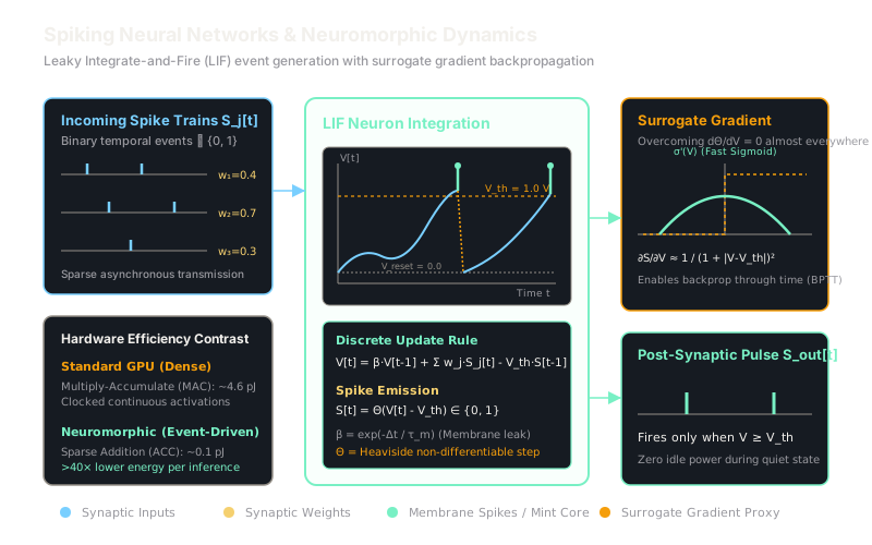
Membrane potential accumulation, threshold spike emission, and exponential leakage in a leaky integrate-and-fire neuron.

Why Does This Exist?

Modern deep learning architectures are power hungry. Training or querying a standard convolutional network or Transformer requires billions of dense Multiply-Accumulate (MAC) floating-point calculations every second. Every neuron computes continuous dot products whether its inputs carry crucial information or static background silence. A high-end GPU dissipates 300 to 700 watts executing synchronized clock cycles for dense tensor arithmetic.

In contrast, biological brains consume roughly 20 watts while outperforming artificial models in real-time sensorimotor control. The key computational difference is temporal sparsity: biological neurons communicate via sparse, asynchronous electrical action potentials called spikes. When no information changes, no spikes occur, and zero dynamic energy is consumed.

Spiking Neural Networks (SNNs) and neuromorphic hardware architectures (such as Intel Loihi, IBM TrueNorth, and SynSense DYNAP) replicate this biological event-driven computing paradigm. In an SNN, floating-point multiplications are replaced by simple additions triggered only when an incoming binary spike arrives. However, training SNNs long remained an open challenge because the threshold firing function is mathematically non-differentiable—its derivative is zero everywhere and infinite at the firing point. Modern SNNs overcome this hurdle via surrogate gradient descent, allowing standard backpropagation through time to optimize biologically plausible models.

Think of It Like This

A drip bucket at a water park playground

Imagine a large decorative tipping bucket mounted over a playground pool.

In a traditional artificial network, a worker stands above the pool constantly pouring a measured stream of water into a pipe every second, while a flow meter measures the exact continuous liters per minute. The pump, pipes, and flow meter run nonstop, drawing massive electrical current even when the water flow barely fluctuates.

A spiking neuron acts like the tipping bucket. Water drips into the bucket from incoming pipes (incoming synaptic currents). At the bottom of the bucket is a tiny leak hole that continuously drains water at a constant rate (membrane leak). If only a few stray drops land in the bucket, the water drains out through the leak hole and the bucket remains stationary.

If a sudden burst of water arrives faster than the leak rate, the bucket fills up, passes its tipping threshold, and suddenly dumps a sharp wave of water down onto the splash pad below (a spike). The bucket instantly resets to completely empty (membrane reset). Downstream buckets react only when that wave splashes into them. When no water flows, everything sits silent, burning zero energy.

How It Actually Works

Leaky Integrate-and-Fire Dynamics and Surrogate Gradients

The standard building block of modern SNNs is the Leaky Integrate-and-Fire (LIF) neuron. Over discrete simulation time steps $t \in \{1, 2, \dots, T\}$ , the sub-threshold membrane potential $V[t]$ is updated using an exponential decay factor $\beta \in (0, 1)$ :

V[t] = \beta V[t-1] + \sum_{j} W_j S_j[t] - V_{\text{th}} S[t-1]

The mathematical terms govern:

$V[t] \in \mathbb{R}$ : The internal membrane potential at time step $t$ .
$\beta = \exp(-\Delta t / \tau_m)$ : The membrane decay factor, where $\tau_m$ is the membrane time constant.
$W_j \in \mathbb{R}$ : The synaptic weight connecting pre-synaptic neuron $j$ to this neuron.
$S_j[t] \in \{0, 1\}$ : The incoming binary spike from pre-synaptic neuron $j$ at time step $t$ .
$V_{\text{th}} \in \mathbb{R}$ : The firing threshold voltage.
$-V_{\text{th}} S[t-1]$ : The reset mechanism (here, soft reset; hard reset forces $V[t] \leftarrow V_{\text{reset}}$ immediately upon firing).

Spike emission is governed by the Heaviside step function $\Theta$ :

S[t] = \Theta(V[t] - V_{\text{th}}) = \begin{cases} 1 & \text{if } V[t] \ge V_{\text{th}} \\ 0 & \text{otherwise} \end{cases}

Because the derivative of the Heaviside step function is the Dirac delta $\delta(V - V_{\text{th}})$ , it evaluates to zero everywhere except at $V = V_{\text{th}}$ , where it is mathematically undefined. Naive backpropagation causes all gradients $\frac{\partial \mathcal{L}}{\partial W}$ to vanish completely.

To train SNNs using standard backpropagation through time (BPTT), we employ surrogate gradients. During the forward pass, the network uses the true discrete step function $\Theta(V - V_{\text{th}})$ . During the backward pass, the non-differentiable step is replaced by a smooth, continuous proxy function, such as the fast sigmoid derivative:

\frac{\partial S}{\partial V} \approx \sigma'(V - V_{\text{th}}) = \frac{1}{\left(1 + \pi |V - V_{\text{th}}|\right)^2}

This surrogate allows gradients to flow smoothly back across temporal states and synaptic weights, enabling end-to-end optimization via standard Adam or SGD.

Worked Example

Consider a single LIF neuron evaluated across $T = 4$ discrete time steps with the following parameters:

Decay factor: $\beta = 0.8$
Firing threshold: $V_{\text{th}} = 1.0\text{ V}$
Reset potential: $V_{\text{reset}} = 0.0\text{ V}$ (using hard reset)
Initial potential: $V[0] = 0.0\text{ V}$
Incoming weighted synaptic input currents $I[t] = \sum_j W_j S_j[t]$ across 4 steps: $I = [0.6, 0.7, 0.2, 0.9]\text{ V}$

Let us trace the membrane potential $V[t]$ and spike outputs $S[t]$ step by step:

Time Step $t = 1$ :

Input current: $I[1] = 0.6\text{ V}$
Membrane potential: $V[1] = \beta V[0] + I[1] = 0.8 \times 0.0 + 0.6 = 0.60\text{ V}$
Threshold check: $0.60 < 1.0 \implies$ No spike fired: $S[1] = 0$ .
Post-step membrane potential: $V[1] = 0.60\text{ V}$ .

Time Step $t = 2$ :

Input current: $I[2] = 0.7\text{ V}$
Membrane potential: $V[2] = \beta V[1] + I[2] = 0.8 \times 0.60 + 0.7 = 0.48 + 0.7 = 1.18\text{ V}$
Threshold check: $1.18 \ge 1.0 \implies$ Spike emitted! $S[2] = 1$ .
Hard reset applied: The membrane potential resets immediately to $V_{\text{reset}} = 0.0\text{ V}$ .

Time Step $t = 3$ :

Input current: $I[3] = 0.2\text{ V}$
Membrane potential: $V[3] = \beta \times 0.0 + 0.2 = 0.20\text{ V}$ (since step 2 reset to 0)
Threshold check: $0.20 < 1.0 \implies$ No spike fired: $S[3] = 0$ .
Post-step membrane potential: $V[3] = 0.20\text{ V}$ .

Time Step $t = 4$ :

Input current: $I[4] = 0.9\text{ V}$
Membrane potential: $V[4] = \beta V[3] + I[4] = 0.8 \times 0.20 + 0.9 = 0.16 + 0.9 = 1.06\text{ V}$
Threshold check: $1.06 \ge 1.0 \implies$ Spike emitted! $S[4] = 1$ .
Hard reset applied: Membrane resets to $0.0\text{ V}$ .

Across 4 time steps, the neuron emitted 2 discrete spikes: $S = [0, 1, 0, 1]$ . On neuromorphic hardware, downstream synapses only computed operations during steps 2 and 4, remaining completely dormant during steps 1 and 3.

Code

Here is a clean PyTorch implementation of an SNN Leaky Integrate-and-Fire layer utilizing a custom surrogate gradient autograd function:

1import torch2import torch.nn as nn3
4
5class FastSigmoidSurrogate(torch.autograd.Function):6    """Custom autograd function: step forward, smooth derivative backward."""7
8    @staticmethod9    def forward(ctx, membrane: torch.Tensor, v_th: float) -> torch.Tensor:10        ctx.save_for_backward(membrane)11        ctx.v_th = v_th12        # True Heaviside step forward13        return (membrane >= v_th).float()14
15    @staticmethod16    def backward(ctx, grad_output: torch.Tensor) -> tuple[torch.Tensor, None]:17        (membrane,) = ctx.saved_tensors18        # Surrogate smooth gradient backward19        v_diff = membrane - ctx.v_th20        surrogate_grad = 1.0 / (1.0 + torch.abs(3.14159 * v_diff)) ** 221        return grad_output * surrogate_grad, None22
23
24class LIFLayer(nn.Module):25    """Leaky Integrate-and-Fire layer with surrogate gradient descent."""26
27    def __init__(self, in_features: int, out_features: int, beta: float = 0.8, v_th: float = 1.0) -> None:28        super().__init__()29        self.beta = beta30        self.v_th = v_th31        self.weights = nn.Linear(in_features, out_features, bias=False)32        self.spike_fn = FastSigmoidSurrogate.apply33
34    def forward(self, spike_sequence: torch.Tensor) -> tuple[torch.Tensor, torch.Tensor]:35        """Processes temporal spike sequence of shape (time_steps, batch_size, in_features)."""36        time_steps, batch_size, _ = spike_sequence.shape37        out_features = self.weights.out_features38
39        v = torch.zeros(batch_size, out_features, device=spike_sequence.device)40        spikes_out = []41
42        for t in range(time_steps):43            # Sparse input current: W * S[t]44            cur_input = self.weights(spike_sequence[t])45            # Leaky integration46            v = self.beta * v + cur_input47            # Spike generation48            s = self.spike_fn(v, self.v_th)49            # Hard reset: zero out potential for fired neurons50            v = v * (1.0 - s)51            spikes_out.append(s)52
53        return torch.stack(spikes_out, dim=0), v54
55
56# Verification run matching worked example57torch.manual_seed(42)58lif = LIFLayer(in_features=1, out_features=1, beta=0.8, v_th=1.0)59with torch.no_grad():60    lif.weights.weight.fill_(1.0)61
62# 4 time steps matching worked example currents: [0.6, 0.7, 0.2, 0.9]63currents = torch.tensor([[[0.6]], [[0.7]], [[0.2]], [[0.9]]])64spikes, final_v = lif(currents)65
66print("Emitted spikes per step:")67for t in range(4):68    print(f"Step {t+1}: {int(spikes[t].item())}")69# -> Step 1: 070# -> Step 2: 171# -> Step 3: 072# -> Step 4: 1

Watch Out For

Dead neurons and vanishing temporal gradients during surrogate backpropagation

A common failure mode in SNN training is the "silent neuron" trap. If the firing threshold $V_{\text{th}}$ is initialized too high relative to input weight scales, neurons rarely or never fire. Because surrogate gradients are localized around $V_{\text{th}}$ , neurons whose membrane potentials never approach $V_{\text{th}}$ receive zero surrogate gradient: $\sigma'(V - V_{\text{th}}) \approx 0$ . The neuron stays dead forever, stalling weight updates.

Conversely, if $V_{\text{th}}$ is set too low, neurons fire indiscriminately on every step, causing severe gradient explosion when backpropagating through long temporal sequences.

Fix: Always normalize input currents using temporal batch normalization (such as Neuromorphic BatchNorm) or scale initial weights using variance scaling adapted to SNN firing rates ( $W \sim \mathcal{N}(0, 2 / (fan_{\text{in}} \cdot V_{\text{th}}))$ ). Additionally, set a loss penalty on target firing rate (e.g., target firing frequency between 5% and 20%) to keep neurons inside the active gradient corridor.

The Quick Version

Spiking Neural Networks exchange sparse binary events ( $\{0, 1\}$ ) instead of continuous floating-point tensors across temporal steps.
On neuromorphic chips, sparse spikes replace expensive floating-point multiply-accumulate (MAC) operations with sparse additions, slashing energy use by over $40\times$ .
The Leaky Integrate-and-Fire (LIF) model integrates incoming charge with an exponential leak until the membrane potential crosses a firing threshold.
Surrogate gradients solve the non-differentiable step function, allowing standard backpropagation through time to train deep SNNs end-to-end.