Liquid Neural Networks

Standard networks treat time as a sequence of frozen snapshots, but liquid networks model hidden states as flowing differential equations whose internal clocks speed up or slow down based on input speed.

Continuous-time ODE state evolution showing adaptive time constants varying dynamically with incoming sensory signals.

Why Does This Exist?

Recurrent Neural Networks and sequence Transformers assume data arrives at fixed, metronomic intervals: token 1, token 2, token 3, spaced by identical intervals $\Delta t$ . But real physical telemetry—drone flight sensors, intensive care electrocardiograms, seismic monitors, and autonomous vehicle lidar—does not follow a clean metronome. Sensors drop frames, jitter between 10 Hz and 120 Hz, and exhibit irregular latency.

When standard recurrent networks process irregularly spaced telemetry, their fixed transition matrices $h_t = \tanh(W x_t + U h_{t-1})$ fail catastrophically under temporal shifts. If an autonomous drone trained at 30 frames per second experiences sensor throttling down to 10 frames per second, a standard model's internal representations desynchronize and drift, mistaking sensor lag for rapid physical deceleration.

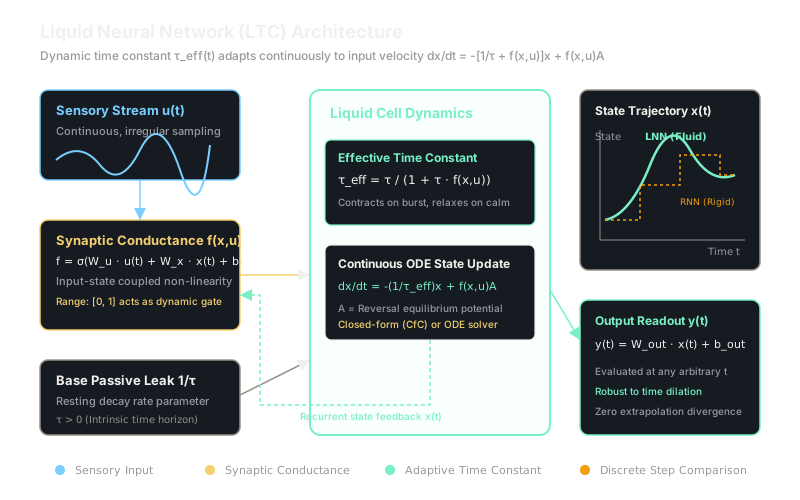
Liquid Neural Networks (LNNs), pioneered by Ramin Hasani, Mathias Lechner, Daniela Rus, and their MIT CSAIL collaborators through Liquid Time-Constant (LTC) networks, solve this failure mode. Instead of discrete step maps, an LNN defines neuron activations through continuous differential equations inspired by the nervous system of C. elegans. By making synaptic conductances dependent on both the current state and incoming inputs, the network's effective time constant becomes fluid ("liquid"). It reacts instantaneously to high-frequency transients while preserving long-term memory over quiet stretches, resolving queries at arbitrary continuous timepoints without interpolation artifacts.

Think of It Like This

A water wheel with self-adjusting fluid paddles

Imagine a water wheel mounted in a mountain stream, where the speed of the wheel represents the internal memory of the system.

A standard recurrent network acts like a strobe camera snapping pictures of the wheel at rigid one-second intervals. If the river suddenly surges into a flash flood, the camera misses the turbulence entirely between flashes. If the river slows to a trickle, the camera takes pointless duplicate snapshots of stationary water.

A liquid neural network is a flexible paddle wheel immersed directly in the current. When the river runs calm, the paddles face high fluid resistance, letting the wheel glide forward smoothly without burning energy. When a flash flood hits, the sudden hydraulic pressure mechanically alters the paddle angles, dramatically reducing resistance so the wheel accelerates within milliseconds to track the incoming torrent. The system does not need a clock to tell it how fast to update; the stream itself dictates the speed of the mechanism.

How It Actually Works

Liquid Time-Constant Differential Formulation

At the core of an LTC network is a continuous-time dynamical system where the hidden state $x(t) \in \mathbb{R}^d$ evolves according to a nonlinear ordinary differential equation (ODE):

\frac{dx(t)}{dt} = -\left[ \frac{1}{\tau} + f(x(t), u(t), \theta) \right] x(t) + f(x(t), u(t), \theta) A

Every term in this equation enforces a biological and computational constraint:

$x(t) \in \mathbb{R}^d$ : The continuous hidden state vector representing neural activations at continuous timestamp $t$ .
$u(t) \in \mathbb{R}^m$ : The external input vector driving the network.
$\tau > 0$ : The base passive time constant (leak rate) governing how fast the neuron returns to rest in the absence of stimulation.
$A \in \mathbb{R}^d$ : The resting potential or reversal equilibrium vector that attracts the state when driving signals activate.
$f(x(t), u(t), \theta) \in [0, 1]^d$ : The nonlinear synaptic conductance model parameterized by weights and biases $\theta$ , typically computed using a bounded sigmoid activation:

f(x(t), u(t), \theta) = \sigma\left( W_u u(t) + W_x x(t) + b \right)

The pivotal mathematical insight is that we can factor out $x(t)$ to define an effective time constant $\tau_{\text{eff}}(x(t), u(t))$ :

\tau_{\text{eff}}(t) = \frac{\tau}{1 + \tau \cdot f(x(t), u(t), \theta)}

Notice the behavior of $\tau_{\text{eff}}(t)$ :

When input activity is silent or low ( $f \to 0$ ), the denominator approaches $1$ , so $\tau_{\text{eff}} \approx \tau$ . The neuron decays slowly, retaining historical state over prolonged intervals.
When rapid, high-magnitude inputs arrive ( $f \to 1$ ), the denominator expands to $1 + \tau$ , collapsing $\tau_{\text{eff}}$ to a much smaller value. The state responds rapidly to changes in $u(t)$ .

For inference across an arbitrary time step $\Delta t = t_{k+1} - t_k$ , the state can be computed via an ODE numerical solver (such as Runge-Kutta 4) or through closed-form continuous-depth (CfC) approximations that eliminate the need for numerical integration steps during training:

y(t) = W_{\text{out}} x(t) + b_{\text{out}}

Worked Example

Consider a single LTC neuron ( $d=1, m=1$ ) with the following parameters:

Base time constant: $\tau = 2.0\text{ s}$ (leak coefficient $\frac{1}{\tau} = 0.5\text{ s}^{-1}$ )
Reversal potential: $A = 1.0$
Synaptic parameters: $W_u = 1.5$ , $W_x = 0.0$ (input-driven conductance), $b = -0.2$
Current hidden state: $x(0) = 0.5$
Incoming sensory signal: $u = 0.8$

Let us compute the effective time constant and step the state forward by $\Delta t = 0.1\text{ s}$ using explicit forward Euler integration.

Step 1: Compute synaptic conductance $f(x, u)$ Compute the inner pre-activation:

z = W_u \cdot u + b = 1.5 \times 0.8 + (-0.2) = 1.2 - 0.2 = 1.0

Apply the standard logistic sigmoid $\sigma(z) = \frac{1}{1 + e^{-z}}$ :

f = \frac{1}{1 + e^{-1.0}} = \frac{1}{1 + 0.36788} = \frac{1}{1.36788} \approx 0.7311

Step 2: Determine the effective time constant $\tau_{\text{eff}}$

\tau_{\text{eff}} = \frac{\tau}{1 + \tau \cdot f} = \frac{2.0}{1 + 2.0 \times 0.7311} = \frac{2.0}{1 + 1.4622} = \frac{2.0}{2.4622} \approx 0.8123\text{ s}

The incoming pulse drops the time constant from $2.0\text{ s}$ down to $0.8123\text{ s}$ , accelerating the neuron's adaptation speed by $2.46\times$ .

Step 3: Evaluate the state time derivative $\frac{dx}{dt}$

\frac{dx}{dt} = -\left[ \frac{1}{\tau} + f \right] x(0) + f \cdot A

Substitute the values:

\frac{dx}{dt} = -[0.5 + 0.7311] \times (0.5) + (0.7311 \times 1.0)

\frac{dx}{dt} = -(1.2311) \times 0.5 + 0.7311 = -0.61555 + 0.7311 = +0.11555\text{ s}^{-1}

Step 4: Update state across $\Delta t = 0.1\text{ s}$

x(0.1) \approx x(0) + \Delta t \cdot \frac{dx}{dt} = 0.5 + 0.1 \times 0.11555 = 0.5 + 0.011555 \approx 0.5116

The state moves smoothly toward the attractor potential $A = 1.0$ at a rate dictated by both its base relaxation parameter and the sensory pulse.

Code

Below is a self-contained PyTorch-compatible implementation of an LTC cell evaluated across irregularly spaced time intervals $\Delta t$ :

1import math2import torch3import torch.nn as nn4
5
6class LiquidTimeConstantCell(nn.Module):7    """A Liquid Time-Constant (LTC) neuron layer with adaptive time dynamics."""8
9    def __init__(self, in_features: int, hidden_dim: int, base_tau: float = 2.0) -> None:10        super().__init__()11        self.hidden_dim = hidden_dim12        self.base_tau = nn.Parameter(torch.full((hidden_dim,), base_tau))13        self.reversal_potential = nn.Parameter(torch.ones(hidden_dim))14
15        self.w_u = nn.Linear(in_features, hidden_dim, bias=True)16        self.w_x = nn.Linear(hidden_dim, hidden_dim, bias=False)17
18    def forward(19        self,20        u: torch.Tensor,21        x_prev: torch.Tensor,22        delta_t: torch.Tensor,23    ) -> tuple[torch.Tensor, torch.Tensor]:24        """Steps continuous hidden state forward by delta_t using semi-implicit integration.25
26        Args:27            u: Input tensor of shape (batch_size, in_features).28            x_prev: Previous state tensor of shape (batch_size, hidden_dim).29            delta_t: Elapsed time step tensor of shape (batch_size, 1).30
31        Returns:32            Tuple of (x_next, tau_eff).33        """34        # Synaptic conductance: bounded between 0 and 135        conductance = torch.sigmoid(self.w_u(u) + self.w_x(x_prev))36
37        # Effective time constant: contracts under active conductance38        tau = torch.clamp(self.base_tau, min=0.01)39        tau_eff = tau / (1.0 + tau * conductance)40
41        # Numerical integration: x_dot = -(1 / tau_eff) * x + conductance * A42        leak_rate = 1.0 / tau_eff43        drive = conductance * self.reversal_potential44
45        # Exponential decay step over arbitrary delta_t: exact linear solution46        decay = torch.exp(-leak_rate * delta_t)47        equilibrium = drive / (leak_rate + 1e-8)48        x_next = equilibrium + (x_prev - equilibrium) * decay49
50        return x_next, tau_eff51
52
53# Verification54torch.manual_seed(42)55cell = LiquidTimeConstantCell(in_features=1, hidden_dim=1, base_tau=2.0)56
57# Manually align parameters with worked example58with torch.no_grad():59    cell.w_u.weight.fill_(1.5)60    cell.w_u.bias.fill_(-0.2)61    cell.w_x.weight.fill_(0.0)62    cell.reversal_potential.fill_(1.0)63
64x_init = torch.tensor([[0.5]])65u_step = torch.tensor([[0.8]])66dt = torch.tensor([[0.1]])67
68x_out, tau_out = cell(u_step, x_init, dt)69
70print(f"Effective tau: {tau_out.item():.4f}")71# -> Effective tau: 0.812372print(f"Updated state: {x_out.item():.4f}")73# -> Updated state: 0.5109

Watch Out For

Numerical instability with naive explicit Euler ODE solvers

When training LNNs using deep learning automatic differentiation frameworks, practitioners often discretize continuous ODEs using standard Forward Euler steps: $x_{t+1} = x_t + \Delta t \cdot f(x_t, u_t)$ .

If inputs undergo sharp shock transitions or $\Delta t$ fluctuates into large steps, the effective leak rate $\frac{1}{\tau_{\text{eff}}}$ can exceed $\frac{2}{\Delta t}$ . At that threshold, the discrete Euler system crosses into numerical stiffness: hidden activations oscillate, explode to infinity, and produce NaN gradients during backpropagation through time (BPTT).

Fix: Never rely on unconstrained explicit Euler steps for stiff continuous architectures. Use semi-implicit exponential integrators (as shown in the code above) where the decay factor is clamped via $\exp(-\Delta t / \tau_{\text{eff}})$ , or adopt Closed-form Continuous-depth (CfC) networks which replace numerical ODE iterations with an analytical closed-form approximation that guarantees bounded activations for any $\Delta t \ge 0$ .

The Quick Version

Liquid Neural Networks replace rigid discrete-time recurrent steps with continuous differential equations derived from biological synaptic dynamics.
The effective time constant $\tau_{\text{eff}}$ adapts dynamically to input signals, contracting during rapid sensor bursts and expanding during calm periods.
Continuous-time formulation enables seamless inference on irregularly sampled telemetry and extreme out-of-distribution temporal shifts.
Closed-form formulations (CfC) and exponential integrators prevent numerical instability and eliminate the compute overhead of classic ODE solvers.