Core ML

CNN Architecture Lineage

One lineage, one fix at a time — from the first working digit classifier to networks a thousand layers deep, then engineered back down to fit a phone.

Each architecture in this lineage fixed one specific limitation of the last: AlexNet proved depth, VGG made it uniform, GoogLeNet cut the parameter cost, and ResNet made real depth trainable at all

Why Does This Exist?

Every architecture on this page exists because a specific, named limitation of its predecessor was blocking progress, and someone found the smallest change that removed it. Read in isolation, each network looks like a fresh design. Read as a sequence, the field's history turns into a series of one-line arguments: this breaks past a certain size, here's the fix, now that's the new limit.

That sequencing is the point of this page. It exists to connect the individual mechanisms — convolution, pooling, and residual connections — to the moment each one got introduced and the specific wall it was answering. Skip the history and every architecture choice in a modern network looks arbitrary. Follow the chain and each one looks inevitable.

Think of It Like This

A relay where each runner fixes what slowed the last one down

A relay team keeps swapping in a new runner, and each new runner isn't just "faster" in the abstract — they're specifically built to fix whatever went wrong on the last leg. One runner ran out of stamina at distance, so the next leg is handed to a specialist in endurance. That specialist was still slow off the blocks, so the leg after that goes to someone built for a fast start.

Nobody designed the whole relay from scratch, in order, ahead of time. Each new leg responded to the specific failure the team had just watched happen. The lineage of CNN architectures reads the same way: LeNet proved the baton could be carried at all, and everything after it is a runner brought in to fix one specific thing that made the previous leg stumble.

How It Actually Works

LeNet (1998) — proof that the shape works at all

Yann LeCun's LeNet-5 was built to read handwritten digits on bank checks: a handful of convolutional and pooling layers, feeding a small classifier. Seven layers, trivial by today's standard, and it worked well enough to see real deployment. Its job in this lineage isn't to be impressive — it's to establish that "convolution, then pooling, repeated, then classify" is a workable shape at all. Everything that follows is a variation on the same skeleton.

AlexNet (2012) — depth and scale, once GPUs made it affordable

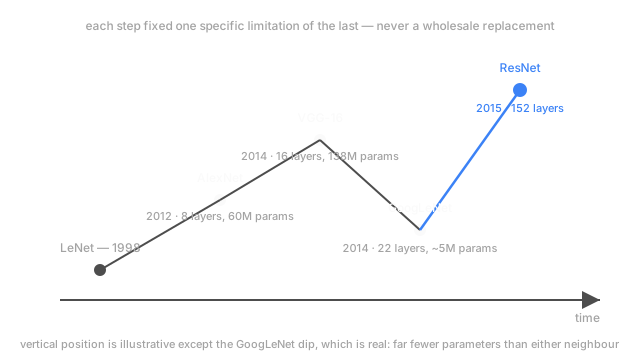
For over a decade after LeNet, deep convolutional networks stayed a research curiosity, mostly because training anything substantially deeper was too slow to be practical. AlexNet's real contribution wasn't a new mechanism — it was proof that training a much deeper network (eight layers, 60 million parameters) on far more data, using GPUs instead of CPUs, produced a decisive jump in accuracy: a 15.3% top-5 error rate on ImageNet, more than ten points ahead of the next-best entry that year. That gap is what convinced the field depth and scale were worth the engineering cost, not an incremental improvement worth footnoting.

VGG (2014) — depth made systematic

AlexNet's specific kernel sizes and layer choices had no obvious underlying rule; they were reasonable engineering judgment calls. VGG's contribution was discipline: use only 3×3 kernels, everywhere, and go deeper by stacking more of that one uniform block rather than varying kernel sizes layer to layer. Receptive field growth from stacked small kernels turns out to match what a single larger kernel would cover, at a fraction of the parameters — the exact arithmetic that page walks through directly.

The cost of that uniformity was sheer parameter count: VGG-16 carries roughly 138 million parameters, more than twice AlexNet's, mostly because it never varies its approach to trade some of that count away.

GoogLeNet / Inception (2014) — the same accuracy, engineered down

GoogLeNet answered VGG's parameter cost directly, and in the same year. Its Inception block runs several differently-shaped convolutions on the same input in parallel — a 1×1, a 3×3, a 5×5 — and concatenates their outputs, rather than committing to one kernel size per layer. Small 1×1 convolutions inside that block, used purely to reduce channel count before the more expensive convolutions run, are the specific trick that keeps the whole thing affordable. The result: roughly 5 million parameters, competitive with VGG's accuracy at well under a tenth of the parameter cost — proof that "more parameters" and "more depth" are not the same lever.

ResNet (2015) — depth stops being the limit at all

Both VGG and GoogLeNet were still shallow compared to what came next. Push a plain stack of convolutional layers much past twenty layers and training accuracy itself degrades — the degradation problem residual connections exists to fix, covered in full on that page. ResNet's identity-plus-correction block made 50, 101, and 152-layer networks not just possible but reliably trainable, and 152-layer ResNet won that year's ImageNet challenge outright. This is the point in the lineage where "how deep can we go" stopped being the open question.

DenseNet, EfficientNet, and ConvNeXt — refining what depth alone can't fix

Once depth was solved, later work asked different questions. DenseNet (2016) connects every layer's output to every later layer's input, not just the next one, on the logic that features should be reusable rather than re-derived at each stage. EfficientNet (2019) asked what to scale, given a fixed compute budget: scaling depth, width, and input resolution together, by a single compound coefficient, out-performed scaling any one dimension alone — a systematic answer to a question earlier architectures had each solved ad hoc. ConvNeXt (2022) is the most recent turn: after vision transformers briefly overtook convolutional networks on major benchmarks, ConvNeXt showed that a purely convolutional network, modernized with design choices borrowed from transformers — larger kernels, different normalization placement, a training recipe update — could match or beat them, without abandoning convolution at all.

Show Me the Code

Not every architecture change is exotic. The GoogLeNet-era trick — using a 1×1 convolution purely to cut channel count before an expensive layer runs — is a few lines, and the parameter savings are directly computable.

1def conv_params(kernel: int, in_ch: int, out_ch: int) -> int:2    return kernel * kernel * in_ch * out_ch  # weights only, no bias3
4
5# A 5x5 conv straight from 256 channels to 256 channels6direct = conv_params(5, 256, 256)7
8# The same job, routed through a 1x1 "bottleneck" that drops to 64 channels first9bottleneck = conv_params(1, 256, 64) + conv_params(5, 64, 64) + conv_params(1, 64, 256)10
11print(f"direct 5x5:        {direct:,}")12print(f"1x1-bottlenecked:  {bottleneck:,}")13print(f"reduction factor:  {direct / bottleneck:.1f}x")14# -> direct 5x5:        1,638,40015# -> 1x1-bottlenecked:  135,16816# -> reduction factor:  12.1x

Twelve times fewer weights for a layer that still ends up mapping 256 channels to 256 channels — the two 1×1 layers cost relatively little themselves, while the expensive 5×5 convolution now only has to operate on 64 channels instead of 256, which is where nearly all of the savings come from.

Watch Out For

Treating 'newer' as a synonym for 'better for your task'

This lineage reads like steady progress, and on the specific benchmark each paper targeted, it mostly was. That doesn't make the newest architecture the right default for an unrelated task. A small, well-labeled dataset for a narrow classification problem often does better with a smaller, older architecture — or a smaller network from this same lineage via transfer learning — than with the largest, newest network, which needs far more data to justify its added capacity and is slower to train and to serve.

Match the architecture's era and scale to your actual data and latency budget, not to whichever name is most recent in the literature.

Assuming every fix in this lineage is additive with every other one

It's tempting to assume you can freely combine every idea in this history — Inception's parallel branches, DenseNet's dense connections, a ResNet-style skip, EfficientNet's compound scaling — into one architecture and get the best of everything. Some combinations compose cleanly; others fight each other over the same compute or memory budget, or duplicate what another already provides. Read what a specific technique was built to fix before assuming it stacks for free with a different one built to fix something else.

The Quick Version

LeNet (1998) proved the convolution-then-pool shape works. AlexNet (2012) proved it works at real depth and scale, once GPUs made that affordable.
VGG (2014) made depth systematic with uniform 3×3 kernels, at the cost of a large parameter count.
GoogLeNet (2014) cut that cost with parallel kernel branches and 1×1 channel-reducing bottlenecks — competitive accuracy at a fraction of the parameters.
ResNet (2015) removed depth itself as the limiting factor, using residual connections to make 100-plus-layer networks reliably trainable.
DenseNet, EfficientNet, and ConvNeXt each answered a narrower question once raw depth was solved: feature reuse, principled scaling, and closing the gap with vision transformers.
Match an architecture's era and scale to your task's actual data and latency budget — newer is not automatically the right choice.