Continuous Normalizing Flows

Instead of stacking discrete invertible neural network layers, continuous normalizing flows let data points drift smoothly along velocity vector fields defined by ordinary differential equations. This continuous flow turns arbitrary data distributions into simple Gaussians while exact probabilities are tracked along the path.

Continuous normalizing flow trajectory governed by a neural ODE velocity field with instantaneous trace integration and adjoint backpropagation

Why Does This Exist?

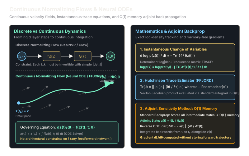
Discrete normalizing flows like RealNVP and Glow obtain tractable likelihoods by constraining layer architectures. To keep Jacobian matrices triangular and readily invertible, models split features into partitions or restrict channel transformations to invertible $1 \times 1$ matrices. These structural handcuffs limit expressive power per layer, forcing practitioners to stack dozens of coupling blocks and store every intermediate activation tensor in GPU memory during backpropagation.

Continuous Normalizing Flows (CNFs), built on Neural Ordinary Differential Equations (Neural ODEs), remove these architectural restrictions. Rather than defining transformations through a discrete chain of layers $z_{k+1} = f_k(z_k)$ , a CNF defines the transformation through a continuous-time differential equation:

\frac{dz(t)}{dt} = f(z(t), t; \theta)

Because any smooth, Lipschitz-continuous vector field produces a bijective, unique trajectory that never crosses itself, the network $f(z(t), t; \theta)$ requires zero architectural constraints. It can be an arbitrary multi-layer perceptron or residual convolutional network. Furthermore, the instantaneous change-of-variables theorem replaces the difficult matrix determinant with a simple matrix trace.

Think of It Like This

Floating downstream through a mountain river

Imagine placing a fleet of toy boats across a wide lake and opening floodgates into a twisting canyon river. Each boat's position changes continuously over time, steered purely by the local water velocity at its exact location.

Because two boats cannot occupy the same water molecule at the same instant, their paths never intersect. As the river flows from time $t_0$ to $t_1$ , the scattered boats gradually gather into a predictable, compact basin. If you want to know where a boat started, simply reverse the river's flow and watch it float backward along its exact trajectory. You never need separate rules for moving forward versus backward—the water's continuous velocity field handles both.

How It Actually Works

Instantaneous Change of Variables and Adjoint Sensitivity

In discrete flows, the density transform requires the full Jacobian determinant:

\log p(z_k) = \log p(z_{k+1}) + \log \left| \det \frac{\partial f_k}{\partial z_k} \right|

In a continuous flow governed by $\frac{dz(t)}{dt} = f(z(t), t; \theta)$ , the continuous counterpart is the instantaneous change of variables formula:

\frac{\partial \log p(z(t))}{\partial t} = -\operatorname{Tr}\left( \frac{\partial f(z(t), t; \theta)}{\partial z(t)} \right)

Integrating this differential equation from data space $t_0$ to prior space $t_1$ yields the total change in log-density:

\log p(x) = \log p(z(t_1)) - \int_{t_0}^{t_1} \operatorname{Tr}\left( \frac{\partial f(z(t), t; \theta)}{\partial z(t)} \right) dt

Computing the exact trace of the $D \times D$ Jacobian matrix $\frac{\partial f}{\partial z}$ normally takes $\mathcal{O}(D^2)$ operations using $D$ vector-Jacobian products. FFJORD (Free-form Jacobian of Reversible Dynamics) scales this to high dimensions using the Hutchinson trace estimator:

\operatorname{Tr}(J) = \mathbb{E}_{p(\epsilon)} \left[ \epsilon^T J \epsilon \right]

where $\epsilon$ is a random noise vector drawn from a standard normal or Rademacher distribution ( $\epsilon_i \in \{-1, +1\}$ with equal probability). By computing $\epsilon^T \left( \frac{\partial f}{\partial z} \right) \epsilon$ , automatic differentiation evaluates the trace in $\mathcal{O}(D)$ operations using a single backward pass.

To optimize parameters $\theta$ without storing all intermediate states along the integration path, the adjoint sensitivity method defines an adjoint state:

a(t) = \frac{\partial L}{\partial z(t)}

The adjoint satisfies its own reverse-time ordinary differential equation:

\frac{da(t)}{dt} = -a(t)^T \frac{\partial f(z(t), t; \theta)}{\partial z(t)}

The loss gradient with respect to model parameters is obtained by integrating backwards from $t_1$ to $t_0$ :

\frac{dL}{d\theta} = -\int_{t_1}^{t_0} a(t)^T \frac{\partial f(z(t), t; \theta)}{\partial \theta} dt

This guarantees $\mathcal{O}(1)$ memory consumption with respect to integration depth, eliminating the activation caching bottleneck of discrete deep networks.

Worked Example

Consider a 2-dimensional continuous flow from $t_0 = 0$ to $t_1 = 1$ . Let the observed data vector be $x = z(0) = [1.0, 2.0]^T$ .

The parameterized vector field is:

f(z(t), t) = \begin{bmatrix} -0.5 z_1 \\ -0.8 z_2 + 0.1 t \end{bmatrix}

The Jacobian is diagonal:

\frac{\partial f}{\partial z} = \begin{bmatrix} -0.5 & 0 \\ 0 & -0.8 \end{bmatrix}, \quad \operatorname{Tr}\left( \frac{\partial f}{\partial z} \right) = -0.5 + (-0.8) = -1.30

Let us numerically integrate using an explicit Euler solver with step size $\Delta t = 0.5$ (2 steps):

First step ( $t = 0 \to 0.5$ ):
- Velocity at $t = 0$ : $f(z(0), 0) = [-0.5(1.0), -0.8(2.0) + 0.1(0)] = [-0.5, -1.6]$
- Position update: $z(0.5) = z(0) + \Delta t \cdot f(z(0), 0) = [1.0, 2.0] + 0.5 \cdot [-0.5, -1.6] = [0.75, 1.20]$
- Instantaneous trace: $\operatorname{Tr}(J) = -1.30$
- Density update: $\Delta \log p_1 = -(-1.30) \times 0.5 = +0.65$
Second step ( $t = 0.5 \to 1.0$ ):
- Velocity at $t = 0.5$ : $f(z(0.5), 0.5) = [-0.5(0.75), -0.8(1.20) + 0.1(0.5)] = [-0.375, -0.910]$
- Position update: $z(1.0) = z(0.5) + \Delta t \cdot f(z(0.5), 0.5) = [0.75, 1.20] + 0.5 \cdot [-0.375, -0.910] = [0.5625, 0.7450]$
- Density update: $\Delta \log p_2 = -(-1.30) \times 0.5 = +0.65$
Total Log-Likelihood:
- Base prior log-density for standard 2D Gaussian $p_{prior}(z) = \frac{1}{2\pi} \exp\left(-\frac{\|z\|^2}{2}\right)$ : $\log p_{prior}(z(1)) = -\log(2\pi) - \frac{0.5625^2 + 0.7450^2}{2} = -1.8379 - 0.4357 = -2.2736$
- Combined data log-likelihood: $\log p(x) = \log p_{prior}(z(1)) + \Delta \log p_1 + \Delta \log p_2 = -2.2736 + 1.30 = -0.9736$

Code

1from typing import Callable, Tuple2import math3
4Vector = list[float]5
6def vector_field(z: Vector, t: float) -> Tuple[Vector, float]:7    """Evaluates dz/dt = f(z, t) and the exact divergence (trace of Jacobian)."""8    dz1 = -0.5 * z[0]9    dz2 = -0.8 * z[1] + 0.1 * t10    trace = -0.5 + (-0.8)11    return [dz1, dz2], trace12
13
14def euler_cnf_step(15    z: Vector, 16    t: float, 17    dt: float, 18    vf: Callable[[Vector, float], Tuple[Vector, float]]19) -> Tuple[Vector, float]:20    """Single forward integration step tracking state and accumulated log-density."""21    dz, trace = vf(z, t)22    z_next = [z[i] + dt * dz[i] for i in range(len(z))]23    d_log_p = -trace * dt24    return z_next, d_log_p25
26
27# Simulate trajectory from t=0.0 to t=1.0 with dt=0.528z_state = [1.0, 2.0]29total_d_log_p = 0.030t_current = 0.031dt = 0.532
33for step in range(2):34    z_state, delta_log_p = euler_cnf_step(z_state, t_current, dt, vector_field)35    total_d_log_p += delta_log_p36    t_current += dt37
38# Compute prior log density under 2D standard Gaussian39norm_sq = z_state[0] ** 2 + z_state[1] ** 240log_p_prior = -math.log(2.0 * math.pi) - 0.5 * norm_sq41log_p_x = log_p_prior + total_d_log_p42
43print("Terminal state z(1):", [round(v, 4) for v in z_state])44# -> Terminal state z(1): [0.5625, 0.745]45print("Log prior p(z):", round(log_p_prior, 4))46# -> Log prior p(z): -2.273647print("Accumulated divergence integral:", round(total_d_log_p, 4))48# -> Accumulated divergence integral: 1.349print("Total data log-likelihood log p(x):", round(log_p_x, 4))50# -> Total data log-likelihood log p(x): -0.9736

Watch Out For

Stiff ODE trajectories causing runaway function evaluations (NFE)

Symptom: Training time per epoch multiplies tenfold over several hundred steps, with adaptive ODE solvers (like Dormand-Prince / dopri5) hanging indefinitely.

As a continuous flow neural network trains without regularization, its learned vector field can develop extreme velocity gradients and turbulent swirls. Adaptive solvers must shrink their integration step sizes $\Delta t$ toward zero to satisfy local error tolerances, causing the Number of Function Evaluations (NFE) to explode from 20 to over 1,000 per sample.

The solution is trajectory regularization. Penalize both the Frobenius norm of the Jacobian and the kinetic energy of the path: $\mathcal{L}_{reg} = \lambda \int_{t_0}^{t_1} \|f(z(t), t)\|^2 dt$ . This straightens the flow paths, enforces smooth dynamics, and keeps NFE small throughout training.

The Quick Version

Continuous Normalizing Flows replace discrete layer stacks with neural vector fields integrated over continuous time.
Any standard feedforward neural network can define the dynamics; invertibility is guaranteed by ODE trajectory uniqueness.
The instantaneous change of variables simplifies log-determinants into the trace of the Jacobian.
Hutchinson's trace estimator approximates the trace in $\mathcal{O}(D)$ operations using random projection vectors.
The adjoint sensitivity method enables exact backpropagation backwards in time with constant $\mathcal{O}(1)$ memory.