Audio and Speech Representations

Sound begins as rapid air pressure waves recorded thousands of times per second. By slicing these raw waveforms into short overlapping windows and calculating their frequency spectrum on a human-inspired Mel scale, models get clear visual-like audio representations.

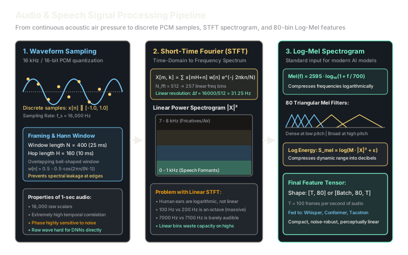
End-to-end audio processing pipeline transforming continuous waveform to PCM samples, STFT spectrogram, and 80-channel log-Mel filterbank

Why Does This Exist?

Feeding raw 1D acoustic audio directly into deep neural networks presents severe statistical hurdles. At a standard speech sampling rate of $16\text{ kHz}$ , a single second of speech contains $16{,}000$ discrete scalar values. A short five-second sentence produces $80{,}000$ timesteps. Adjacent waveform samples are dominated by phase information and microscopic air-pressure oscillations that shift drastically if a speaker moves half an inch from the microphone, even though the phoneme spoken remains identical.

Directly processing raw audio in the time domain forces neural networks to expend massive capacity learning basic Fourier-like filters from scratch. Furthermore, human auditory perception does not perceive acoustic frequency linearly. The human cochlea resolves pitch with exquisite precision in low frequencies below $1\text{ kHz}$ (where speech formants distinguish vowels like "aa" vs "ee"), while grouping frequencies above $4\text{ kHz}$ into coarse perceptual bands.

Transforming 1D waveforms into 2D time-frequency representations—most notably the Short-Time Fourier Transform (STFT) and Log-Mel Spectrogram—compresses high-rate audio into compact matrices of approximately 100 frames per second, isolating invariant phonetic content from noisy acoustic phase.

Think of It Like This

A musical score transcribed from live violin vibrations

Imagine placing a high-speed camera in front of a violin string vibrating 440 times per second ( $440\text{ Hz}$ ). If you record the vertical position of the string at every microsecond, you get an overwhelming list of millions of raw numbers that obscure the tune.

Instead, a composer listens in short fractions of a second and marks which musical note is sounding on a sheet music staff. The vertical axis on the staff represents the pitch (arranged so that higher octaves space out naturally to the human ear), the horizontal axis represents time, and the darkness of the note represents loudness. A Mel spectrogram is simply automated sheet music for machines: it strips away the raw mechanical string flutter and leaves only the melody, harmonics, and rhythm.

How It Actually Works

From Continuous Waves to Log-Mel Spectrograms

The standard audio feature extraction pipeline proceeds through four distinct mathematical stages:

1. Sampling and Quantization (Nyquist-Shannon Theorem)

Continuous acoustic pressure $x(t)$ is converted to a discrete sequence $x[n] = x(n \cdot T_s)$ where $T_s = 1/f_s$ . By the Nyquist-Shannon sampling theorem, capturing frequencies up to $f_{\text{max}}$ requires a sampling rate $f_s \ge 2 f_{\text{max}}$ . For standard human speech (bandwidth up to $8\text{ kHz}$ ), $f_s = 16{,}000\text{ Hz}$ is the universal standard. Samples are quantized into 16-bit signed integers (PCM format) spanning $[-32768, 32767]$ and normalized to $[-1.0, 1.0]$ .

2. Framing and Windowing

Speech signals are non-stationary over long intervals, but quasi-stationary over short windows of $20\text{ to }30\text{ ms}$ (the physical speed at which human vocal cords and articulators change shape). The signal is partitioned into overlapping frames of length $N = 400$ ( $25\text{ ms}$ at $16\text{ kHz}$ ) with hop size $H = 160$ ( $10\text{ ms}$ ). To prevent spectral leakage caused by abruptly truncating waveforms at frame boundaries, each frame is multiplied by a bell-shaped Hann window $w[n]$ :

w[n] = 0.5 - 0.5 \cos\left( \frac{2\pi n}{N - 1} \right), \quad 0 \le n \le N-1

3. Short-Time Fourier Transform (STFT)

For each windowed frame $m$ , an $N_{\text{fft}}$ -point Fast Fourier Transform (typically $N_{\text{fft}} = 512$ ) computes the discrete complex spectrum:

X[m, k] = \sum_{n=0}^{N-1} x[m \cdot H + n] \cdot w[n] \cdot e^{-j \frac{2\pi k n}{N_{\text{fft}}}}, \quad 0 \le k \le \frac{N_{\text{fft}}}{2}

Because real-valued signals yield conjugate-symmetric spectra, only the first $N_{\text{fft}}/2 + 1 = 257$ frequency bins are retained. The power spectrogram is the squared magnitude:

P[m, k] = |X[m, k]|^2 = \operatorname{Re}(X[m, k])^2 + \operatorname{Im}(X[m, k])^2

4. Mel Filterbank Integration and Log Compression

The linear frequency $f$ in Hertz is mapped to the perceptual Mel scale $m$ via:

m = 2595 \log_{10}\left(1 + \frac{f}{700}\right)

A bank of $M$ overlapping triangular filters (typically $M = 80$ for models like Whisper) spans from $0\text{ Hz}$ to $f_s/2 = 8000\text{ Hz}$ . Each filter $H_i[k]$ computes a weighted sum over the linear power bins:

S_{\text{mel}}[m, i] = \sum_{k=0}^{N_{\text{fft}}/2} P[m, k] \cdot H_i[k], \quad 1 \le i \le M

Finally, human perception of loudness is logarithmic (measured in decibels). Applying a logarithm with numerical offset $\epsilon$ produces the final Log-Mel Spectrogram:

Y[m, i] = \log(S_{\text{mel}}[m, i] + \epsilon)

Worked Example

Let us trace the frequency-to-mel mapping and STFT bin assignment for a speech signal recorded at $f_s = 16{,}000\text{ Hz}$ with $N_{\text{fft}} = 512$ bins and $M = 80$ filters.

Calculate Linear Bin Spacing: $\Delta f = \frac{f_s}{N_{\text{fft}}} = \frac{16000}{512} = 31.25\text{ Hz per bin}$
Locate a $400\text{ Hz}$ Fundamental Pitch: $k = \frac{400}{\Delta f} = \frac{400}{31.25} = 12.8 \implies \text{Bin index } 13$
Convert Linear Frequencies to Mel Scale:
- At $f = 400\text{ Hz}$ (first vowel formant): $m(400) = 2595 \log_{10}\left(1 + \frac{400}{700}\right) = 2595 \log_{10}(1.5714) = 2595 \times 0.1963 = 509.4\text{ mels}$
- At $f = 800\text{ Hz}$ (second harmonic): $m(800) = 2595 \log_{10}\left(1 + \frac{800}{700}\right) = 2595 \log_{10}(2.1429) = 2595 \times 0.3310 = 859.0\text{ mels}$
- At $f = 1600\text{ Hz}$ (third harmonic): $m(1600) = 2595 \log_{10}\left(1 + \frac{1600}{700}\right) = 2595 \log_{10}(3.2857) = 2595 \times 0.5166 = 1340.6\text{ mels}$
Observe Non-Linear Compression:
- Interval $400\text{ Hz} \to 800\text{ Hz}$ span: $859.0 - 509.4 = 349.6\text{ mels}$
- Interval $800\text{ Hz} \to 1600\text{ Hz}$ span: $1340.6 - 859.0 = 481.6\text{ mels}$ The doubling from 800 to 1600 Hz covers only 1.38x the perceptual distance of 400 to 800 Hz, concentrating filterbank resolution where human phoneme distinctions occur.

Code

1from typing import List, Tuple2import math3
4def hz_to_mel(hz: float) -> float:5    """Converts frequency in Hertz to perceptual Mel scale."""6    return 2595.0 * math.log10(1.0 + hz / 700.0)7
8
9def mel_to_hz(mel: float) -> float:10    """Converts perceptual Mel scale back to Hertz."""11    return 700.0 * (10.0 ** (mel / 2595.0) - 1.0)12
13
14def generate_mel_filterbank_centers(15    num_filters: int, 16    f_min: float, 17    f_max: float18) -> List[float]:19    """Computes peak frequencies (Hz) for linearly spaced Mel filters."""20    mel_min = hz_to_mel(f_min)21    mel_max = hz_to_mel(f_max)22    step = (mel_max - mel_min) / (num_filters + 1)23    mel_points = [mel_min + i * step for i in range(1, num_filters + 1)]24    return [mel_to_hz(m) for m in mel_points]25
26
27# Compute filter center frequencies for standard 16 kHz audio setup28centers_hz = generate_mel_filterbank_centers(num_filters=5, f_min=0.0, f_max=8000.0)29
30print("Mel filter center frequencies (Hz):")31for idx, freq in enumerate(centers_hz, 1):32    print(f"Filter {idx}: {freq:.1f} Hz")33# -> Mel filter center frequencies (Hz):34# -> Filter 1: 342.3 Hz35# -> Filter 2: 875.9 Hz36# -> Filter 3: 1707.9 Hz37# -> Filter 4: 3005.1 Hz38# -> Filter 5: 5027.6 Hz39
40# Notice how spacing widens:41diffs = [centers_hz[i+1] - centers_hz[i] for i in range(len(centers_hz)-1)]42print("Bandwidth gaps:", [round(d, 1) for d in diffs])43# -> Bandwidth gaps: [533.6, 832.0, 1297.2, 2022.5]

Watch Out For

Phase erasure during spectrogram synthesis without neural vocoders

Symptom: Audio generated by inverting spectrograms with Griffin-Lim sounds robotic, hollow, or metallic with severe background phase buzzing.

The short-time Fourier transform produces complex values $X[m, k] = |X| e^{j \phi}$ . Converting to power and Mel filterbanks discards the phase $\phi$ completely. The classical Griffin-Lim algorithm iteratively estimates missing phase through repeated forward and inverse STFTs, but it converges slowly and generates distinct metallic artifacts.

In modern generative pipelines (such as text-to-speech or audio super-resolution), never rely on naive phase reconstruction algorithms. Always pair Mel spectrogram generation with a trained neural vocoder (such as HiFi-GAN, WaveNet, or BigVGAN) that learns the non-linear prior distribution of phase directly from data.

The Quick Version

Raw acoustic audio at $16\text{ kHz}$ has high redundancy, noise sensitivity, and massive temporal length ( $16{,}000$ points/sec).
Short-Time Fourier Transform (STFT) windows raw audio into $25\text{ ms}$ frames to extract localized frequency spectra.
The Mel scale aligns frequency bin resolution with human ear cochlear sensitivity, emphasizing lower speech formants.
Overlapping triangular Mel filters followed by logarithmic power compression produce the standard 80-bin Log-Mel spectrogram.
Log-Mel representations are standard inputs for modern speech recognition models like Whisper and speech synthesizers like Tacotron.