Modern Speech and Audio Architectures

Modern audio architectures evolved from dilated convolutions predicting individual sound samples to self-supervised transformers and neural codec language models. Whether converting text into natural voices, transcribing multilingual speech, or cloning voices with tokens, these models treat sound as structured sequences.

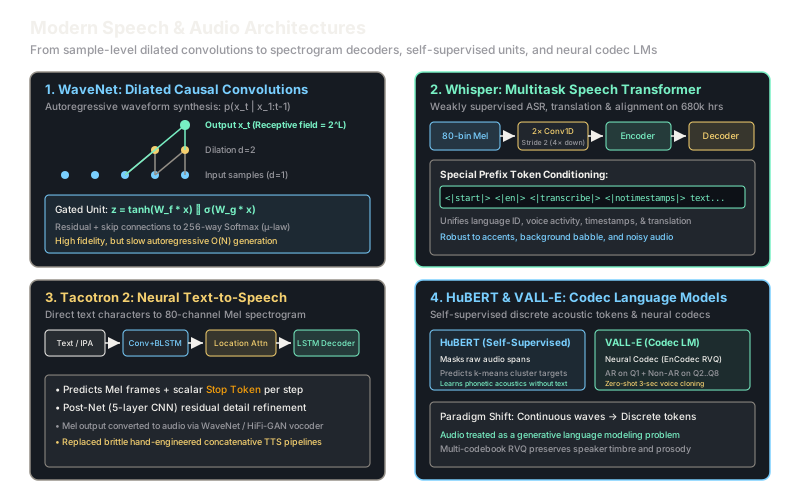
Four landmark audio architectures: WaveNet dilated convolutions, Whisper multitask encoder-decoder, Tacotron TTS, and VALL-E neural codec language model

Why Does This Exist?

For decades, automated speech recognition (ASR) and text-to-speech (TTS) relied on complex, hand-engineered statistical pipelines. Speech recognition coupled acoustic hidden Markov models (HMMs), Gaussian mixture models (GMMs), pronunciation lexicons, and n-gram language models. Speech synthesis concatenated recorded diphones or ran statistical parametric vocoders that produced flat, buzzy, mechanical audio. Each submodule was trained in isolation under different objectives, accumulating compounding errors across pipeline boundaries.

The deep learning revolution transformed audio processing into end-to-end differentiable sequence modeling. Over the past decade, four milestone architectural paradigms emerged:

WaveNet (2016): Proved neural networks can generate raw acoustic waveforms directly using causal dilated convolutions.
Tacotron 2 (2018): Eliminated phoneme alignment pipelines by generating 80-bin Mel spectrograms directly from raw text characters via attention.
Whisper (2022): Showed that scaling a standard encoder-decoder Transformer across 680,000 hours of weakly supervised audio matches human-level robustness across transcription, translation, and voice activity detection without task-specific heads.
HuBERT & VALL-E (2021–2023): Discretized continuous audio into acoustic and semantic tokens via self-supervision and neural codecs (like EnCodec), framing speech synthesis as pure generative language modeling.

Think of It Like This

From hand-painted flipbooks to digital video tokens

Early speech systems were like artists manually assembling a flipbook: one specialist sketched phoneme outlines, another colored the pitch contours, and a third glued the pages together. If any hand slipped, the motion looked jagged and robotic.

WaveNet replaced the flipbook by calculating the exact shade of every microscopic pixel sequentially at 16,000 frames per second. Tacotron stepped back to render the high-level scene composition (the spectrogram) in one stroke. Whisper built an omniscient translator that watches any video stream, ignores background cafe noise, and outputs subtitles in 99 languages. Finally, VALL-E compressed the video into standardized Lego bricks (discrete acoustic tokens), allowing an ordinary text language model to clone anyone's voice from just three seconds of sample audio simply by continuing the sequence.

How It Actually Works

The Four Landmark Paradigms

1. WaveNet: Dilated Causal Convolutions

WaveNet models the joint probability of an audio waveform $x = \{x_1, x_2, \dots, x_T\}$ as a product of conditional probabilities:

p(x) = \prod_{t=1}^T p(x_t \mid x_1, x_2, \dots, x_{t-1})

To prevent future samples from leaking into the past, convolutions are strictly causal. Standard convolutions require thousands of layers to cover hundreds of milliseconds of audio. WaveNet introduces dilated convolutions, where filters skip input values with dilation factor $d$ . By doubling dilation exponentially across layers ( $d \in \{1, 2, 4, 8, \dots, 512\}$ ), the receptive field grows exponentially with network depth while computational complexity scales linearly:

\text{Receptive Field} = 1 + (k - 1) \sum_{l=0}^{L-1} 2^l = 1 + (k - 1)(2^L - 1)

Each layer applies a gated activation unit modeled after PixelCNN:

z = \tanh(W_{f,k} * x) \odot \sigma(W_{g,k} * x)

where $W_{f,k}$ and $W_{g,k}$ denote filter and gate convolutions, and $\odot$ is element-wise multiplication.

2. Tacotron 2: Attention-Based Spectrogram Synthesis

Tacotron 2 maps text character sequences to Mel spectrogram frames. It consists of:

Encoder: Character embeddings pass through a 3-layer convolutional filterbank followed by a Bidirectional LSTM to extract contextual phonemic representations.
Location-Sensitive Attention: Computes alignment weights using both the decoder state and previous cumulative attention weights, preventing phoneme repetitions and omissions.
Autoregressive Decoder: A 2-layer unidirectional LSTM that predicts one 80-bin Mel frame $y_t$ alongside a scalar stop token (trained via binary cross-entropy) indicating end-of-speech.
Post-Net: A 5-layer convolutional network that predicts a residual detail tensor added to the decoder output, minimizing mean squared error before feeding into a neural vocoder.

3. Whisper: Weakly Supervised Multitask Transformer

OpenAI's Whisper formats all speech tasks (ASR, speech translation, voice activity detection, and word-level alignment) as sequence-to-sequence language modeling:

Input Representation: 80-channel Log-Mel spectrogram computed with $25\text{ ms}$ windows and $10\text{ ms}$ hops.
Stem: Two 1D convolutional layers with filter width 3 and stride 2 downsample the temporal dimension by a factor of 4.
Encoder-Decoder Transformer: Standard sinusoidal position embeddings feed a Transformer encoder. The autoregressive decoder receives special prefix conditioning tokens:

[\langle|\text{startoftranscript}|\rangle, \langle|\text{language}|\rangle, \langle|\text{task}|\rangle, \langle|\text{notimestamps}|\rangle, \dots \text{tokens}]

Conditioning on tokens like $\langle|\text{translate}|\rangle$ switches the decoder from transcription to English translation without changing a single model parameter.

4. HuBERT & VALL-E: Discrete Acoustic Units and Codec LMs

HuBERT (Hidden-Unit BERT): Takes continuous audio, applies span masking, and trains a BERT-like encoder to predict discrete cluster IDs obtained from $k$ -means clustering on intermediate feature representations. This forces the model to learn phonemic abstractions without human transcriptions.
VALL-E: Uses a neural audio codec (EnCodec) that compresses $24\text{ kHz}$ audio into 8 hierarchical codebooks via Residual Vector Quantization (RVQ) at 75 tokens per second. An autoregressive language model generates the first codebook tokens $c_1$ conditioned on phoneme text and a 3-second acoustic prompt. Then, a non-autoregressive Transformer predicts codebooks $c_2$ through $c_8$ in parallel, achieving zero-shot voice cloning.

Worked Example

Let us compare the receptive field and computational scaling between WaveNet and Whisper.

WaveNet Exponential Receptive Field:
- Kernel size $k = 2$ .
- Dilation cycle: 10 layers with $d = [1, 2, 4, 8, 16, 32, 64, 128, 256, 512]$ .
- Receptive field per 10-layer block: $R = 1 + (2 - 1) \times (2^{10} - 1) = 1 + 1023 = 1024\text{ samples}$
- Stacking 3 repeating cycles ( $L = 30$ layers total): $R_{\text{total}} = 1 + 3 \times 1023 = 3070\text{ samples}$
- At a $16\text{ kHz}$ sampling rate ( $16\text{ samples/ms}$ ): $T_{\text{receptive}} = \frac{3070}{16000} \approx 0.1919\text{ seconds } (191.9\text{ ms})$
- Captures approximately two syllables of speech context without any pooling layers.
Whisper Conv1D Stem Temporal Downsampling:
- Input audio: $30\text{ seconds}$ at $16\text{ kHz} = 480{,}000$ waveform samples.
- Mel spectrogram frames ( $10\text{ ms}$ hop): $T_{\text{mel}} = \frac{30}{0.010} = 3000\text{ frames}$
- Two Conv1D layers with stride 2 downsample time by $2 \times 2 = 4\times$ : $T_{\text{transformer}} = \frac{3000}{4} = 750\text{ sequence length}$
- Full self-attention matrix comparisons drop from $3000^2 = 9{,}000{,}000$ to $750^2 = 562{,}500$ operations—a $16\times$ computation reduction that makes 30-second context windows practical on standard GPUs.

Code

1from typing import List2
3def wavenet_receptive_field(kernel_size: int, dilations: List[int], stacks: int) -> int:4    """Calculates the exact theoretical receptive field of a stacked WaveNet."""5    single_stack_field = sum(d * (kernel_size - 1) for d in dilations)6    return 1 + stacks * single_stack_field7
8
9def whisper_sequence_length(duration_sec: float, hop_ms: float, strides: List[int]) -> int:10    """Calculates downsampled Transformer sequence length in Whisper."""11    num_mel_frames = int((duration_sec * 1000.0) / hop_ms)12    total_downsample = 113    for s in strides:14        total_downsample *= s15    return num_mel_frames // total_downsample16
17
18# 1. Evaluate WaveNet with 3 stacks of 10 dilated layers19dil_pattern = [2**i for i in range(10)]  # [1, 2, 4, ..., 512]20rf_samples = wavenet_receptive_field(kernel_size=2, dilations=dil_pattern, stacks=3)21duration_ms = (rf_samples / 16000.0) * 1000.022
23print(f"WaveNet Receptive Field: {rf_samples} samples ({duration_ms:.1f} ms)")24# -> WaveNet Receptive Field: 3070 samples (191.9 ms)25
26# 2. Evaluate Whisper 30-second audio window downsampling27seq_len = whisper_sequence_length(duration_sec=30.0, hop_ms=10.0, strides=[2, 2])28print(f"Whisper Transformer Sequence Length: {seq_len} tokens")29# -> Whisper Transformer Sequence Length: 750 tokens

Watch Out For

Autoregressive generation latency in sample-level vocoders

Symptom: A speech synthesis model takes 45 seconds of GPU computation to generate just 3 seconds of spoken audio, rendering it useless for interactive voice assistants.

Because WaveNet predicts raw audio sample-by-sample, generating 3 seconds of audio at $24\text{ kHz}$ requires $72{,}000$ sequential forward passes through the network. Even with optimized CUDA caching, sequential inference cannot saturate GPU tensor cores.

Modern production pipelines decouple semantic generation from audio rendering. Use FastSpeech 2 or VALL-E to generate Mel frames or discrete codec tokens in parallel, and synthesize raw waveforms using non-autoregressive GAN vocoders like HiFi-GAN or diffusion vocoders like DiffWave, which render entire audio clips in a single forward pass with $0.05\times$ real-time factor.

The Quick Version

WaveNet proved that dilated causal convolutions can synthesize raw audio waveforms sample-by-sample without pooling.
Tacotron 2 eliminated multi-stage TTS pipelines by using attention to map text directly to 80-channel Mel spectrograms.
Whisper scales standard encoder-decoder Transformers across 680,000 hours, unifying speech tasks via special prefix tokens.
HuBERT uses masked prediction of k-means cluster targets to learn rich phonetic representations without text transcriptions.
VALL-E and modern codec models treat audio as discrete tokens, turning zero-shot speech generation into a language modeling problem.