DeepWalk and Node2Vec
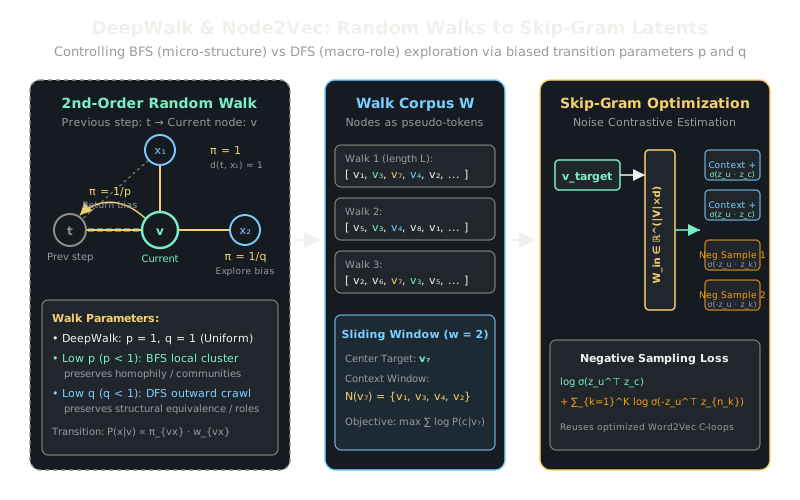
DeepWalk and Node2Vec simulate random walks across a network to turn graphs into sequences of nodes trained like sentences in language models.
Why Does This Exist?
In the early 2010s, natural language processing experienced a revolution when Word2Vec revealed that dense word representations could be learned efficiently by sliding context windows over text sentences. Graph practitioners wanted similar continuous embeddings for network nodes, but graphs lack a natural sequential ordering: there is no single "beginning", "middle", or "end" to a graph topology.
Computing global pairwise distances across millions of nodes using matrix factorization algorithms (like spectral decomposition of the Laplacian) incurs an intractable or computational cost and collapses when graph edges evolve. DeepWalk (Perozzi et al., 2014) solved this by realizing that truncated random walks on a network exhibit the exact same power-law frequency distribution as words in natural language corpora. Node2Vec (Grover & Leskovec, 2016) generalized DeepWalk by introducing parameterized, second-order random walks that allow practitioners to interpolate smoothly between local community clustering (homophily) and structural network roles (such as hubs or bridges).
Think of It Like This
A wandering tourist exploring a foreign city
Imagine a tourist landing in an unfamiliar historic city with narrow alleys, ring roads, and town squares. If the tourist strolls by flipping a fair coin at every crossroad, taking 40 steps before stopping, their trip diary records a sequence of street corners. Two corners that sit along the same bustling avenue will frequently appear adjacent in those diary entries.
Now give the tourist a guidebook with two dial knobs:
- The Return knob () controls homesickness. Set it low, and the tourist loves looping back to where they just came from, thoroughly mapping out the tiny alleys of their immediate neighborhood (Breadth-First Search).
- The Exploration knob () controls adventurousness. Set it low, and the tourist avoids turning around, charging straight outward across major avenues into foreign districts to discover how far the city reaches (Depth-First Search).
Feeding thousands of these tourist journals into a text model teaches it which landmarks share a local neighborhood and which act as structural city gates.
How It Actually Works
2nd-Order Biased Walks and Skip-Gram Objective
Node2Vec defines a flexible neighborhood for every node by simulating second-order random walks. Suppose a walk just traversed edge and is currently positioned at node . The probability of taking the next step to a neighbor is:
The unnormalized transition probability is the product of the edge weight and a search bias :
The search bias depends on the shortest-path distance between the previous node and candidate neighbor :
- Return parameter : High () discourages revisiting recent nodes, reducing 2-hop redundancy. Low () forces the walk to stay local, emulating Breadth-First Search (BFS) to capture homophily (nodes in the same community get similar embeddings).
- In-out parameter : Low () encourages the walk to venture outward, emulating Depth-First Search (DFS) to capture structural equivalence (nodes serving identical topological roles, like hubs or peripheral leaves, get similar embeddings regardless of distance).
- DeepWalk Equivalence: Setting and recovers the uniform random walk of DeepWalk.
Once a corpus of random walks is generated, the embeddings are optimized using the Skip-Gram architecture with Negative Sampling:
where is the center representation of node , is the context representation of neighbor , , and is the number of negative samples drawn from noise distribution .
Worked Example
Let a walk transition from to . The neighbors of are :
- : distance .
- : edge exists in the graph, so distance .
- : no edge between and , so distance .
Assume unweighted edges (), return parameter , and in-out parameter :
-
Calculate unnormalized biases :
-
Compute normalization denominator :
-
Compute exact transition probabilities:
Because and , the walker is more likely to double back to than to step out toward distant node , heavily favoring local community clustering.
Code
import randomfrom typing import Dict, List
def sample_node2vec_step( prev_node: int, curr_node: int, adjacency: Dict[int, List[int]], p: float, q: float,) -> int: """Sample next node in 2nd-order biased random walk given (prev_node, curr_node).""" neighbors = adjacency[curr_node] prev_neighbors = set(adjacency[prev_node])
weights: List[float] = [] for nbr in neighbors: if nbr == prev_node: # d(prev, nbr) == 0 weights.append(1.0 / p) elif nbr in prev_neighbors: # d(prev, nbr) == 1 (mutual neighbor) weights.append(1.0) else: # d(prev, nbr) == 2 (outward step) weights.append(1.0 / q)
# Weighted random sampling chosen: int = random.choices(neighbors, weights=weights, k=1)[0] return chosen
# Test with graph: 0-1, 1-2 (with edge 0-2), 1-3 (no edge 0-3)adj: Dict[int, List[int]] = { 0: [1, 2], 1: [0, 2, 3], 2: [0, 1], 3: [1],}
# Fix seed for reproducible checkrandom.seed(42)counts: Dict[int, int] = {0: 0, 2: 0, 3: 0}for _ in range(10_000): nxt = sample_node2vec_step(prev_node=0, curr_node=1, adjacency=adj, p=0.5, q=2.0) counts[nxt] += 1
# Node 0 (return) ~57%, Node 2 (mutual) ~28%, Node 3 (outward) ~14%print(f"Empirical distribution: 0: {counts[0]/10000:.3f}, 2: {counts[2]/10000:.3f}, 3: {counts[3]/10000:.3f}")# -> Empirical distribution: 0: 0.573, 2: 0.285, 3: 0.142Watch Out For
Second-order transition memory explosion
In standard first-order random walks (DeepWalk), transition probabilities only depend on the current node , needing total probability storage. In Node2Vec, the next step depends on the ordered edge pair , which expands memory requirements to where is the average degree.
On large-scale graphs with power-law hubs (where a single celebrity or payment router has edges), precomputing and storing alias tables for every incoming edge will trigger Out-Of-Memory (OOM) errors. For graphs exceeding edges, compute transition weights dynamically on the fly during the random walk or clip maximum neighborhood degrees before preprocessing.
The Quick Version
- DeepWalk transforms graphs into text sequences by generating uniform random walks, applying Skip-Gram with Negative Sampling to learn continuous node vectors.
- Node2Vec introduces second-order walk biases controlled by two hyperparameters: return parameter and exploration parameter .
- Setting prioritizes Breadth-First Search (BFS) to preserve local community homophily, while prioritizes Depth-First Search (DFS) to learn structural network roles.