Message Passing Neural Networks

Message Passing Neural Networks let graph nodes iteratively exchange vector messages with immediate neighbors to update their internal representations.

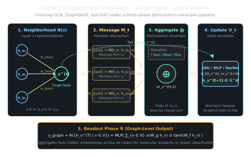
MPNN unifies graph neural networks into three modular phases: message generation along edges, permutation-invariant aggregation, and node state updating

Why Does This Exist?

Between 2015 and 2017, the machine learning literature was flooded with competing graph deep learning architectures: Graph Convolutional Networks (Kipf & Welling), GraphSAGE (Hamilton et al.), Molecular Graph Convolutions (Duvenaud et al.), and Gated Graph Neural Networks (Li et al.). Each used different terminology, notation, and tensor operations, making it difficult to understand whether these models were fundamentally distinct architectures or minor variations of the same underlying principle.

Gilmer et al. (2017) cut through this fragmentation by introducing the Message Passing Neural Network (MPNN) framework. MPNN demonstrated that nearly all spatial graph neural networks are instances of a single elegant computational paradigm: an iterative message exchange between neighboring nodes. Furthermore, MPNN proved that by formalizing these operations, one can guarantee permutation equivariance (reordering node indices produces an identically reordered output) and permutation invariance (predicting a whole-graph property like molecular solubility is completely independent of the arbitrary order in which nodes are indexed).

Think of It Like This

A round-table discussion among department liaisons

Imagine an organization where team managers sit in individual offices connected by telephone lines. Each manager holds a private notepad summarizing their department's current status.

At the top of the hour, every manager executes three steps:

Compose Messages: For every connected colleague, the manager drafts a targeted briefing memo based on what they know and the specific nature of their partnership.
Collect Inboxes: Each manager receives the memos delivered to their door. Because memos arrive simultaneously, the manager stacks them into an inbox without caring which courier dropped off their letter first. They tally or average the figures across all memos.
Update Notes: The manager reads the aggregated briefing summary, compares it against their own previous status notepad, and writes a revised status entry.

After one round of calls, every manager knows what their immediate neighbors know (1-hop awareness). After two rounds, news from two offices away has diffused across the organization (2-hop awareness).

How It Actually Works

The Three Phases: Message, Aggregate, and Update

An MPNN operates on a graph $G = (V, E)$ where nodes possess hidden states $\mathbf{h}_v \in \mathbb{R}^{d_v}$ and edges possess optional feature attributes $\mathbf{e}_{uv} \in \mathbb{R}^{d_e}$ . The forward pass repeats over $T$ discrete message-passing time steps.

Each step $t \in \{1, \dots, T\}$ consists of three algebraic phases:

1. Message Phase

For every directed edge $(u, v) \in E$ , a parameterized message function $M_t$ computes an outgoing message vector $\mathbf{m}_{uv}^{(t)}$ from the source node state $\mathbf{h}_u^{(t-1)}$ , destination state $\mathbf{h}_v^{(t-1)}$ , and edge attributes $\mathbf{e}_{uv}$ :

$\mathbf{m}_{uv}^{(t)} = M_t\left(\mathbf{h}_v^{(t-1)}, \mathbf{h}_u^{(t-1)}, \mathbf{e}_{uv}\right)$

In Graph Convolutional Networks (GCN), $M_t$ is a scaled linear projection: $M_t = \frac{1}{\sqrt{\deg(v)\deg(u)}} \mathbf{W}^{(t)} \mathbf{h}_u$ . In Graph Attention Networks (GAT), $M_t = \alpha_{uv}^{(t)} \mathbf{W}^{(t)} \mathbf{h}_u$ .

2. Aggregation Phase

Node $v$ gathers incoming messages from all adjacent nodes in its neighborhood $\mathcal{N}(v)$ using a permutation-invariant reduction operator $\bigoplus \in \{\sum, \text{mean}, \max\}$ :

$\mathbf{m}_v^{(t)} = \bigoplus_{u \in \mathcal{N}(v)} \mathbf{m}_{uv}^{(t)}$

Because $\bigoplus$ satisfies commutativity ( $a \oplus b = b \oplus a$ ) and associativity ( $(a \oplus b) \oplus c = a \oplus (b \oplus c)$ ), the aggregated message $\mathbf{m}_v^{(t)}$ is strictly invariant to node permutation.

3. Update Phase

The updated node representation $\mathbf{h}_v^{(t)}$ is computed by an update function $U_t$ combining the node's prior state with the aggregated incoming message:

$\mathbf{h}_v^{(t)} = U_t\left(\mathbf{h}_v^{(t-1)}, \mathbf{m}_v^{(t)}\right)$

Common choices for $U_t$ include a Gated Recurrent Unit (GRU cell in GGNN) or a Multi-Layer Perceptron with a residual connection: $\sigma(\mathbf{W}_{\text{self}} \mathbf{h}_v^{(t-1)} + \mathbf{m}_v^{(t)})$ .

4. Readout Phase

For graph-level prediction tasks (e.g., predicting chemical toxicity), a permutation-invariant readout function $R$ pools all final representations $\mathbf{h}_v^{(T)}$ :

$\hat{\mathbf{y}} = R\left(\{\mathbf{h}_v^{(T)} \mid v \in V\}\right) = \text{MLP}\left( \sum_{v \in V} \sigma(\mathbf{W}_g \mathbf{h}_v^{(T)}) \odot \tanh(\mathbf{W}_f \mathbf{h}_v^{(T)}) \right)$

Worked Example

Let node $v$ have two neighbors $u_1$ and $u_2$ . Features are 2-dimensional ( $d = 2$ ).

Initial states: $\mathbf{h}_v^{(0)} = \begin{bmatrix} 1.0 \\ 0.0 \end{bmatrix}, \quad \mathbf{h}_{u_1}^{(0)} = \begin{bmatrix} 0.5 \\ 1.0 \end{bmatrix}, \quad \mathbf{h}_{u_2}^{(0)} = \begin{bmatrix} -0.5 \\ 0.5 \end{bmatrix}$
Linear message weight matrix $\mathbf{W}_M \in \mathbb{R}^{2 \times 2}$ : $\mathbf{W}_M = \begin{bmatrix} 0.5 & 0.0 \\ 0.0 & 0.5 \end{bmatrix}$
Aggregator: $\bigoplus = \sum$ (Sum).
Update function: $U(\mathbf{h}_v, \mathbf{m}_v) = \text{ReLU}(\mathbf{W}_U \mathbf{h}_v + \mathbf{m}_v)$ with $\mathbf{W}_U = \begin{bmatrix} 1.0 & 0.0 \\ 0.0 & 1.0 \end{bmatrix}$ .

Compute Messages: $\mathbf{m}_{u_1 v}^{(1)} = \mathbf{W}_M \mathbf{h}_{u_1}^{(0)} = \begin{bmatrix} 0.5 \times 0.5 \\ 0.5 \times 1.0 \end{bmatrix} = \begin{bmatrix} 0.25 \\ 0.50 \end{bmatrix}$ $\mathbf{m}_{u_2 v}^{(1)} = \mathbf{W}_M \mathbf{h}_{u_2}^{(0)} = \begin{bmatrix} 0.5 \times (-0.5) \\ 0.5 \times 0.5 \end{bmatrix} = \begin{bmatrix} -0.25 \\ 0.25 \end{bmatrix}$
Aggregate Messages: $\mathbf{m}_v^{(1)} = \mathbf{m}_{u_1 v}^{(1)} + \mathbf{m}_{u_2 v}^{(1)} = \begin{bmatrix} 0.25 + (-0.25) \\ 0.50 + 0.25 \end{bmatrix} = \begin{bmatrix} 0.00 \\ 0.75 \end{bmatrix}$
Update State: $\mathbf{z}_v = \mathbf{W}_U \mathbf{h}_v^{(0)} + \mathbf{m}_v^{(1)} = \begin{bmatrix} 1.0 \\ 0.0 \end{bmatrix} + \begin{bmatrix} 0.00 \\ 0.75 \end{bmatrix} = \begin{bmatrix} 1.00 \\ 0.75 \end{bmatrix}$ $\mathbf{h}_v^{(1)} = \text{ReLU}\left(\begin{bmatrix} 1.00 \\ 0.75 \end{bmatrix}\right) = \begin{bmatrix} 1.00 \\ 0.75 \end{bmatrix}$ Node $v$ incorporated structural information from both neighbors while retaining its identity.

Code

1from typing import List, Tuple2import numpy as np3
4
5class MPNNLayer:6    """Minimal single-step Message Passing Neural Network layer."""7
8    def __init__(self, in_dim: int, out_dim: int) -> None:9        rng = np.random.default_rng(seed=42)10        # Message transform matrix11        self.W_msg: np.ndarray = rng.standard_normal((in_dim, out_dim)) * 0.212        # Self-update transform matrix13        self.W_self: np.ndarray = rng.standard_normal((in_dim, out_dim)) * 0.214
15    def forward(16        self,17        node_features: np.ndarray,  # Shape: (N, in_dim)18        edge_index: List[Tuple[int, int]],  # List of directed (src, dst) edges19    ) -> np.ndarray:20        num_nodes = node_features.shape[0]21        out_dim = self.W_msg.shape[1]22
23        # 1. Message Phase: Compute message from each src to dst24        # 2. Aggregation Phase: Sum into accumulator25        aggregated_messages = np.zeros((num_nodes, out_dim), dtype=np.float64)26        for src, dst in edge_index:27            msg = np.dot(node_features[src], self.W_msg)28            aggregated_messages[dst] += msg29
30        # 3. Update Phase: Combine self state with incoming messages + ReLU31        self_transformed = np.dot(node_features, self.W_self)32        updated_states = np.maximum(0.0, self_transformed + aggregated_messages)33        return updated_states34
35
36# Graph: Triangle where 0 <-> 1, 1 <-> 2, 2 <-> 037edges: List[Tuple[int, int]] = [38    (0, 1), (1, 0),39    (1, 2), (2, 1),40    (2, 0), (0, 2),41]42features = np.array([43    [1.0, 0.0],44    [0.5, 1.0],45    [-0.5, 0.5],46], dtype=np.float64)47
48layer = MPNNLayer(in_dim=2, out_dim=2)49out_h = layer.forward(features, edges)50print("Updated node embeddings shape:", out_h.shape)51# -> Updated node embeddings shape: (3, 2)52print("Node 0 new state:", np.round(out_h[0], 4))

Watch Out For

The 1-Weisfeiler-Lehman expressivity bottleneck

Standard MPNN message passing with anonymous node aggregations is theoretically bounded in expressive power by the 1-Weisfeiler-Lehman (1-WL) graph isomorphism test (Morris et al., 2019). An MPNN cannot distinguish between strongly regular graphs that share identical degree distributions and local neighbor multiset structures, such as two disconnected triangles versus one 6-cycle ring.

If your problem domain requires detecting specific molecular substructures (like benzene rings, cliques, or cycles) that 1-WL fails to separate, do not simply stack more MPNN layers. Incorporate structural cycle features, relative random walk positional encodings, or higher-order Subgraph/Cellular GNN architectures.

The Quick Version

MPNN provides a unifying three-stage framework for spatial graph neural networks: Message computation, Aggregation, and State Update.
Permutation equivariance is guaranteed by selecting commutative and associative aggregation operators such as sum, mean, or max.
The theoretical expressive power of standard MPNNs is bounded by the 1-Weisfeiler-Lehman graph isomorphism test.