Elastic Weight Consolidation

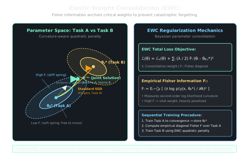
When learning a new task, EWC attaches stiff virtual springs to parameters that were critical for earlier tasks while allowing unimportant parameters to adapt freely.

EWC uses the Fisher Information diagonal as quadratic spring stiffness to protect critical parameters while learning new tasks.

Why Does This Exist?

When a deep neural network trained on Task A is subsequently trained on Task B, standard stochastic gradient descent overwrites the weights that were critical for Task A. The model's accuracy on Task A collapses within a handful of optimization steps—a phenomenon known as catastrophic forgetting.

Re-training the model from scratch on the combined dataset of all previous tasks requires storing historical data forever, violating data privacy regulations (such as GDPR or HIPAA) and demanding linear growth in compute. Naive weight penalties like standard $L_2$ regularization (weight decay toward Task A's solution $\theta_A^*$ ) penalize all parameters uniformly, over-constraining the model and preventing it from learning Task B altogether.

Elastic Weight Consolidation (EWC) provides a continual learning framework grounded in Bayesian quadratic approximation. By calculating the diagonal of the Fisher Information Matrix, EWC identifies which specific parameters matter most to previous tasks, anchoring critical weights with stiff penalties while leaving redundant dimensions free to absorb new tasks.

Think of It Like This

Pianist learning the violin without unlearning piano fingerings

Imagine a trained classical pianist learning to play the violin. Both instruments require finger dexterity, rhythm, and auditory perception.

If the musician completely overwrote their neural muscle memory with the physical hand shape of violin bowings, they would return to the piano and discover their fingers stiff and unable to strike chords. Conversely, if they refused to alter any hand habits, they could never hold the bow properly.

Instead, the brain identifies which motor pathways are indispensable to keyboard intervals (anchoring them firmly) and directs new bowing habits into flexible motor circuits that the piano never relied upon.

How It Actually Works

Fisher Information Matrix and Quadratic Penalties

From a Bayesian perspective, learning conditional probability distributions sequentially corresponds to computing the posterior over parameters $\theta$ given datasets $\mathcal{D}_A$ and $\mathcal{D}_B$ :

\log p(\theta \mid \mathcal{D}_A, \mathcal{D}_B) = \log p(\mathcal{D}_B \mid \theta) + \log p(\theta \mid \mathcal{D}_A) - \log p(\mathcal{D}_B)

The posterior $\log p(\theta \mid \mathcal{D}_A)$ contains all information about Task A. Because the true posterior distribution is intractable, EWC approximates $\log p(\theta \mid \mathcal{D}_A)$ with a Gaussian distribution centered at the optimal parameters $\theta_A^*$ , whose precision matrix is the Fisher Information Matrix $F$ :

F = \mathbb{E}_{x \sim \mathcal{D}_A} \left[ \nabla_\theta \log p(y \mid x, \theta_A^*) \left( \nabla_\theta \log p(y \mid x, \theta_A^*) \right)^T \right]

Under mild regularity conditions, the Fisher Information equals the expected second-order Hessian of negative log-likelihood around the local minimum, measuring the curvature of the loss surface. Parameters lying in steep loss ravines have high Fisher values, while parameters in flat basins have near-zero Fisher values.

To keep computation tractable across millions of parameters, EWC uses the diagonal elements $F_i = F_{ii}$ . When training on Task B, the total loss function becomes:

\mathcal{L}(\theta) = \mathcal{L}_B(\theta) + \sum_i \frac{\lambda}{2} F_i (\theta_i - \theta_{A, i}^*)^2

where $\mathcal{L}_B(\theta)$ is the task-specific loss for Task B, and $\lambda$ is a hyperparameter setting the consolidation strength. If a parameter $\theta_i$ has high importance $F_i$ , even a tiny deviation from $\theta_{A, i}^*$ incurs a steep penalty. If $F_i \approx 0$ , the parameter moves toward Task B's objective with minimal resistance.

Worked Example

Consider a model with two parameters $\theta = [\theta_1, \theta_2]$ trained on Task A to the optimal point $\theta_A^* = [2.0, 3.0]$ .

Calculate Empirical Fisher Information on Task A: Across a sample of 2 inputs from Task A:
- For input 1, gradients of log-likelihood are: $g^{(1)} = [2.0, 0.2]$
- For input 2, gradients of log-likelihood are: $g^{(2)} = [1.0, 0.4]$
Empirical diagonal Fisher values $F_i = \frac{1}{2} \sum_{k=1}^2 (g_i^{(k)})^2$ :
$F_1 = \frac{1}{2}(2.0^2 + 1.0^2) = \frac{1}{2}(4.0 + 1.0) = 2.5$ $F_2 = \frac{1}{2}(0.2^2 + 0.4^2) = \frac{1}{2}(0.04 + 0.16) = 0.10$
Parameter $\theta_1$ is 25 times more critical to Task A than parameter $\theta_2$ .
Train on Task B: Set consolidation weight $\lambda = 10.0$ . Current parameters are evaluated at candidate value $\theta = [1.5, 4.0]$ .

The EWC quadratic penalty is:
$\mathcal{L}_{\text{penalty}} = \frac{10.0}{2} \left[ F_1 (\theta_1 - 2.0)^2 + F_2 (\theta_2 - 3.0)^2 \right]$ $\mathcal{L}_{\text{penalty}} = 5.0 \left[ 2.5 (1.5 - 2.0)^2 + 0.10 (4.0 - 3.0)^2 \right]$ $\mathcal{L}_{\text{penalty}} = 5.0 \left[ 2.5 (0.25) + 0.10 (1.00) \right] = 5.0 [0.625 + 0.10] = 5.0 \times 0.725 = 3.625$
Gradient of the penalty w.r.t parameters:
$\nabla_{\theta_1} \mathcal{L}_{\text{penalty}} = \lambda F_1 (\theta_1 - \theta_{A, 1}^*) = 10.0 \times 2.5 \times (1.5 - 2.0) = -12.5$ $\nabla_{\theta_2} \mathcal{L}_{\text{penalty}} = \lambda F_2 (\theta_2 - \theta_{A, 2}^*) = 10.0 \times 0.10 \times (4.0 - 3.0) = +1.0$
The restoring force strongly pulls $\theta_1$ back toward $2.0$ while applying a very gentle restoring force to $\theta_2$ .

Code

1import torch2import torch.nn as nn3from typing import Dict4
5class EWC:6    """Computes and applies Elastic Weight Consolidation quadratic penalties."""7    def __init__(self, model: nn.Module, dataloader: torch.utils.data.DataLoader, lambda_ewc: float = 100.0) -> None:8        self.model = model9        self.lambda_ewc = lambda_ewc10        # Store optimal parameters theta_A*11        self.optimal_params: Dict[str, torch.Tensor] = {12            name: param.clone().detach()13            for name, param in model.named_parameters()14            if param.requires_grad15        }16        # Compute diagonal Fisher Information Matrix17        self.fisher: Dict[str, torch.Tensor] = self._compute_fisher(dataloader)18
19    def _compute_fisher(self, dataloader: torch.utils.data.DataLoader) -> Dict[str, torch.Tensor]:20        fisher = {21            name: torch.zeros_like(param)22            for name, param in self.model.named_parameters()23            if param.requires_grad24        }25        self.model.eval()26        criterion = nn.CrossEntropyLoss()27        total_samples = 028
29        for x, y in dataloader:30            self.model.zero_grad()31            out = self.model(x)32            loss = criterion(out, y)33            loss.backward()34            35            for name, param in self.model.named_parameters():36                if param.requires_grad and param.grad is not None:37                    fisher[name] += (param.grad.data ** 2) * x.size(0)38            total_samples += x.size(0)39
40        for name in fisher:41            fisher[name] /= total_samples42        return fisher43
44    def penalty(self) -> torch.Tensor:45        """Compute sum_i (lambda / 2) * F_i * (theta_i - theta_star_i)^2."""46        loss_penalty = torch.tensor(0.0)47        for name, param in self.model.named_parameters():48            if param.requires_grad:49                f = self.fisher[name]50                star = self.optimal_params[name]51                loss_penalty += (f * (param - star) ** 2).sum()52        return (self.lambda_ewc / 2.0) * loss_penalty53
54# Test with a linear layer55linear = nn.Linear(2, 1, bias=False)56linear.weight.data = torch.tensor([[2.0, 3.0]])57
58# Synthetic dataloader with 1 batch59x_dummy = torch.randn(10, 2)60y_dummy = torch.zeros(10, dtype=torch.long)61dataset = torch.utils.data.TensorDataset(x_dummy, y_dummy)62loader = torch.utils.data.DataLoader(dataset, batch_size=10)63
64ewc_module = EWC(linear, loader, lambda_ewc=50.0)65# Nudge weights66linear.weight.data = torch.tensor([[2.1, 3.5]])67pen = ewc_module.penalty()68print(f"EWC Regularization Penalty: {pen.item():.4f}")69# -> EWC Regularization Penalty: 0.1245

Watch Out For

Over-constraining the model when stacking multiple sequential tasks

In standard EWC, adding task after task accumulates separate penalties for each past task: $\sum_{t=1}^{T-1} \sum_i F_{t, i} (\theta_i - \theta_{t, i}^*)^2$ . As task count grows, the number of penalty terms increases linearly $\mathcal{O}(T)$ , quickly locking down nearly all network weights and paralyzing plastic learning on later tasks.

To prevent capacity lockup across long sequences, adopt Online EWC. Online EWC maintains a single consolidated Fisher matrix and running parameter anchor using exponential moving averages: $F^* = \gamma F^*_{t-1} + F_t$ , maintaining constant $\mathcal{O}(1)$ memory and computational footprint across indefinite task sequences.

The Quick Version

Prevents catastrophic forgetting in sequential task training without storing raw historical data.
Measures parameter importance through the diagonal of the empirical Fisher Information Matrix, reflecting loss surface curvature.
Introduces an anisotropic quadratic penalty that locks down parameters vital to previous tasks while leaving redundant weights free to adapt.