Experience Replay Architectures

Instead of learning directly from experiences as they happen, an agent stores its memories in a buffer and reviews them in random shuffled batches so it does not get trapped in local feedback loops.

Experience replay decorrelates consecutive transitions via uniform buffers and prioritizes unexpected experiences using sum-tree heaps.

Why Does This Exist?

In standard reinforcement learning, an agent collects consecutive transitions $(s_t, a_t, r_t, s_{t+1})$ sequentially in real time. Training a deep neural network directly on this live stream violates the foundational assumption of stochastic gradient descent: that training samples are independent and identically distributed (i.i.d.).

Consecutive states are strongly autocorrelated: an agent driving a car on a highway observes consecutive video frames that are $99\%$ identical. When gradients from nearly identical states update the network weights consecutively, the model overfits to the immediate local corridor, causing parameter oscillation or catastrophic policy divergence. Furthermore, rare critical events (like hitting an obstacle or collecting a sparse bonus) are experienced once and immediately discarded, causing the network to forget them before sufficient gradient signal propagates backward.

Experience Replay stores transitions into a sliding memory buffer and draws randomized mini-batches for optimization. This simple mechanism breaks temporal correlation, restores i.i.d. sampling assumptions, and allows the agent to reuse rare experiences multiple times across its training lifetime.

Think of It Like This

Studying for a medical licensing exam with flashcards

Imagine a medical student attending emergency room rounds. On Monday, five consecutive patients present with broken ankles; on Tuesday, four consecutive patients arrive with allergic rashes.

If the student studied only the most recent patient in real time, on Monday evening they would prescribe ankle splints for every symptom, and by Tuesday evening they would prescribe antihistamines for broken bones. The sequence of clinical encounters is biased by time and coincidence.

Instead, the student writes each patient's symptoms and diagnosis onto a flashcard and drops it into a study box. Every evening, they shuffle the box thoroughly, pull out twenty random cards from across the past six months, and quiz themselves. Rare cases like venomous snakebites are marked with bright flags and reviewed more frequently than trivial common colds.

How It Actually Works

Temporal Decorrelation and Sum-Tree Prioritization

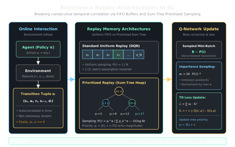
At each environment step $t$ , the agent stores transition tuple $e_t = (s_t, a_t, r_t, s_{t+1}, d_t)$ into a replay memory $\mathcal{D} = \{e_1, \dots, e_N\}$ of capacity $N$ (often $10^5$ to $10^6$ transitions). When capacity is exceeded, the oldest transition is evicted in first-in, first-out (FIFO) order.

In standard Uniform Replay, transitions are sampled uniformly at random $P(i) = \frac{1}{N}$ . This decorrelates consecutive samples, ensuring $\text{Cov}(e_t, e_{t+k}) \approx 0$ within each optimization batch.

However, uniform sampling wastes compute: transitions where the agent already predicts the outcome accurately provide near-zero gradient signal, while rare, highly surprising transitions are sampled no more often than mundane steps.

Prioritized Experience Replay (PER) samples transitions in proportion to their temporal difference (TD) error magnitude $|\delta_i|$ :

\delta_i = r_i + \gamma \max_{a'} Q(s'_i, a'; \theta^-) - Q(s_i, a_i; \theta)

The probability of sampling transition $i$ is defined as:

P(i) = \frac{p_i^\alpha}{\sum_{k} p_k^\alpha}

where priority $p_i = |\delta_i| + \epsilon$ (with small $\epsilon > 0$ preventing zero-probability starvation), and $\alpha \in [0, 1]$ controls prioritization strength ( $\alpha = 0$ is uniform sampling; $\alpha = 1$ is pure greedy prioritization).

Because prioritizing samples alters the visitation frequency of the state distribution, it introduces estimation bias into the Q-learning expected value. PER corrects this bias using Importance Sampling (IS) weights:

w_i = \left( \frac{1}{N} \cdot \frac{1}{P(i)} \right)^\beta

where $\beta \in [0, 1]$ anneals from a small value up to $1.0$ at the end of training. Weights are normalized by $1 / \max_i w_i$ so that updates only scale downward.

To maintain $\mathcal{O}(\log N)$ sampling and update speed instead of an $\mathcal{O}(N)$ linear scan, PER implements a binary Sum-Tree:

Every leaf node stores transition priority $p_i^\alpha$ .
Every internal parent node stores the sum of its two child nodes: $\text{parent} = \text{child}_{\text{left}} + \text{child}_{\text{right}}$ .
The root node holds the total sum $p_{\text{total}} = \sum_k p_k^\alpha$ .
Sampling partitions $[0, p_{\text{total}}]$ into $K$ equal intervals and performs binary search down the tree in $\mathcal{O}(\log N)$ time.

Worked Example

Trace a mini Sum-Tree with 4 leaf transitions holding priorities: $p = [2.0, 6.0, 4.0, 8.0]$ , with $\alpha = 1.0$ , buffer size $N = 4$ , and bias correction $\beta = 0.5$ .

Sum-Tree Structure:
- Leaves: $L_0 = 2.0$ , $L_1 = 6.0$ , $L_2 = 4.0$ , $L_3 = 8.0$ .
- Intermediate nodes: $Node_A = 2.0 + 6.0 = 8.0$ , $Node_B = 4.0 + 8.0 = 12.0$ .
- Root node: $Total = Node_A + Node_B = 8.0 + 12.0 = 20.0$ .
Sampling Probabilities:
$P(0) = \frac{2}{20} = 0.10, \quad P(1) = \frac{6}{20} = 0.30, \quad P(2) = \frac{4}{20} = 0.20, \quad P(3) = \frac{8}{20} = 0.40$
Sample with random query value $v = 11.5$ :
- At Root ( $20.0$ ), check left child $Node_A$ ( $8.0$ ). Since $11.5 > 8.0$ , descend to right child $Node_B$ and subtract left sum: $v' = 11.5 - 8.0 = 3.5$ .
- At $Node_B$ ( $12.0$ ), check left leaf $L_2$ ( $4.0$ ). Since $3.5 \le 4.0$ , descend to left child $L_2$ .
- Leaf chosen: index 2 (priority 4.0).
Compute Importance Sampling Weight for index 2:
$w_2 = (N \cdot P(2))^{-\beta} = (4 \times 0.20)^{-0.5} = (0.8)^{-0.5} \approx 1.118$
For the minimum probability transition (index 0, $P(0) = 0.10$ ):
$w_0 = (4 \times 0.10)^{-0.5} = (0.4)^{-0.5} \approx 1.581$
Normalized weight:
$\bar{w}_2 = \frac{w_2}{w_{\max}} = \frac{1.118}{1.581} \approx 0.707$
The high-priority transition update is scaled down by $0.707$ to correct the sampling bias.

Code

1import numpy as np2from typing import Tuple, List3
4class SumTree:5    """Binary Sum-Tree storing priorities in O(log N) lookup and update."""6    def __init__(self, capacity: int) -> None:7        self.capacity = capacity8        # Tree array: parents occupy 1 to capacity-1, leaves occupy capacity to 2*capacity-19        self.tree = np.zeros(2 * capacity, dtype=np.float32)10        self.data_pointer = 011
12    def add(self, priority: float) -> int:13        tree_idx = self.data_pointer + self.capacity14        self.update(tree_idx, priority)15        data_idx = self.data_pointer16        self.data_pointer = (self.data_pointer + 1) % self.capacity17        return tree_idx18
19    def update(self, tree_idx: int, priority: float) -> None:20        change = priority - self.tree[tree_idx]21        self.tree[tree_idx] = priority22        # Propagate changes up to root23        parent = tree_idx // 224        while parent >= 1:25            self.tree[parent] += change26            parent //= 227
28    def total_priority(self) -> float:29        return float(self.tree[1])30
31    def get_leaf(self, value: float) -> Tuple[int, float]:32        idx = 133        while idx < self.capacity:34            left = 2 * idx35            right = left + 136            if value <= self.tree[left]:37                idx = left38            else:39                value -= self.tree[left]40                idx = right41        return idx, float(self.tree[idx])42
43# Demonstrate O(log N) priority sampling44tree = SumTree(capacity=4)45tree.add(2.0)  # idx 446tree.add(6.0)  # idx 547tree.add(4.0)  # idx 648tree.add(8.0)  # idx 749
50print(f"Total Priority in Root: {tree.total_priority():.1f}")51# Sample with value 11.552leaf_idx, prio = tree.get_leaf(11.5)53data_idx = leaf_idx - tree.capacity54print(f"Sampled Leaf Index: {leaf_idx}, Data Index: {data_idx}, Priority: {prio:.1f}")55# -> Total Priority in Root: 20.056# -> Sampled Leaf Index: 6, Data Index: 2, Priority: 4.0

Watch Out For

Buffer staleness under rapidly evolving target policies

As the Q-network trains over millions of steps, old transitions stored near the bottom of a large buffer ( $N = 10^6$ ) were collected by an exploratory, highly suboptimal policy $\pi_{\text{old}}$ . If sampled alongside fresh transitions without discount adjustments, off-policy divergence can destabilize deep Q-learning.

To mitigate buffer staleness, dynamically scale the buffer size relative to the learning rate, or implement multi-step targets $n$ -step returns with $Q(\lambda)$ or Retrace correction. When using Prioritized Replay, recalculate each transition's TD error $\delta_i$ immediately after each backward pass and refresh its tree priority.

The Quick Version

Eliminates autocorrelation across sequential environment steps, restoring i.i.d. conditions necessary for stable gradient descent.
Prioritized Experience Replay focuses learning capacity on surprising transitions with large TD errors.
Sum-Tree binary heap enables $\mathcal{O}(\log N)$ sampling and priority updates, while Importance Sampling weights prevent parameter estimation bias.