FedAvg and FedProx

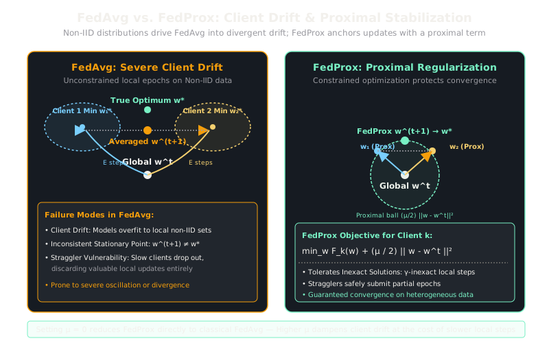
FedAvg lets devices train independently for several steps before averaging their models, but when local data distributions diverge, FedProx adds an elastic leash to keep devices from wandering off course.

FedAvg suffers from client drift on non-IID distributions, while FedProx adds a proximal regularization term to stabilize local updates.

Why Does This Exist?

In distributed edge training, communicating model parameters across high-latency wireless networks is orders of magnitude slower than local GPU computation. If edge devices synchronize with a central server after every single gradient batch (distributed synchronous SGD), training grinds to a halt under network round-trip overhead.

To save bandwidth, Federated Averaging (FedAvg) allows selected edge clients to execute multiple local training epochs before communicating. While FedAvg converges smoothly when clients hold identically distributed (IID) data, real-world edge data is heavily non-IID: users type different slang, hospitals serve distinct demographic cohorts, and cameras record differing lighting conditions.

Under non-IID distributions, each client's local loss function points toward a radically different local optimum. When clients run many local gradient steps without synchronization, their weights wander far apart—a failure mode known as client drift. Averaging drifted weights produces a model that performs poorly on all clients. Furthermore, FedAvg assumes every client finishes the assigned epochs, forcing the system to discard slow "straggler" devices. FedProx was created to fix both flaws.

Think of It Like This

A search party tied together with elastic ropes

Imagine a team of searchers looking for lost hikers across a foggy mountain range. Each searcher holds an outdated map showing different local landmarks.

Under the FedAvg strategy, searchers meet at basecamp, agree on a heading, and then sprint off in their own directions for three full hours before regrouping. Because their local maps differ, searcher A runs deep down into an eastern canyon, while searcher B climbs high onto a western peak. When they return and calculate the average midpoint of their final coordinates, they find themselves standing on an inaccessible cliff where none of them intended to go.

FedProx ties every searcher to the current basecamp with an elastic bungee cord. The searchers can still explore local valleys, but as they wander further away, the tension in the cord pulls them back. They uncover local clues without straying into divergent territory.

How It Actually Works

Client Drift and the Proximal Regularization Term

In federated optimization, the global problem is to minimize:

\min_w f(w) = \sum_{k=1}^K p_k F_k(w) \quad \text{where} \quad p_k = \frac{n_k}{n} \ge 0, \quad \sum_{k=1}^K p_k = 1

In classical FedAvg, each selected client $k$ initializes $w_k^0 = w^t$ and performs $E$ local epochs using standard SGD:

w_k^{j+1} = w_k^j - \eta \nabla F_k(w_k^j)

The server aggregates the terminal weights $w^{t+1} = \sum_k p_k w_k^E$ . When local distributions are heterogeneous ( $F_i(w) \ne F_j(w)$ ), the local minima $w_i^* = \arg\min F_i(w)$ do not align with global minimum $w^* = \arg\min f(w)$ . As $E$ increases, client drift pushes local weights toward individual minima $w_k^*$ , causing the aggregated update to oscillate or diverge.

FedProx stabilizes local training by adding a proximal regularization term to each client's local loss function:

\min_w h_k(w; w^t) = F_k(w) + \frac{\mu}{2} \left\| w - w^t \right\|^2

where:

$w^t$ is the current global model broadcast by the server at the beginning of round $t$ .
$\mu \ge 0$ is a tuning parameter controlling the stiffness of the proximal penalty.
When $\mu = 0$ , FedProx is mathematically identical to FedAvg.
When $\mu > 0$ , the quadratic penalty restricts how far local parameters can deviate from $w^t$ , effectively keeping local updates bounded within a neighborhood where the global direction remains valid.

In addition to curbing client drift, FedProx formally supports $\gamma$ -inexact solutions. Instead of requiring every client to complete a fixed number of epochs $E$ , clients perform variable amounts of local work depending on their current compute and battery status:

\left\| \nabla h_k(w_k^{t+1}; w^t) \right\| \le \gamma \left\| \nabla h_k(w^t; w^t) \right\|

This allows slow stragglers to contribute partial local progress rather than being dropped entirely from the round.

Worked Example

Consider a 1D parameter $w$ across two clients with non-IID quadratic loss objectives:

Client 1 objective: $F_1(w) = \frac{1}{2}(w - 0)^2 \implies \text{minimum at } w_1^* = 0.0$
Client 2 objective: $F_2(w) = \frac{1}{2}(w - 10)^2 \implies \text{minimum at } w_2^* = 10.0$
Equal dataset sizes ( $p_1 = p_2 = 0.5$ ).
True global objective: $f(w) = \frac{1}{2}[F_1(w) + F_2(w)] \implies \text{true optimum at } w^* = 5.0$ .

Suppose the current global model is $w^t = 2.0$ .

FedAvg (with large local steps to convergence):
- Client 1 minimizes $F_1(w)$ completely: $w_1 = 0.0$ .
- Client 2 minimizes $F_2(w)$ completely: $w_2 = 10.0$ .
- Server average: $w^{t+1} = 0.5(0.0) + 0.5(10.0) = 5.0$
(While symmetric 1D quadratics land at 5.0 in one round, non-convex landscapes with learning rates overshoot and diverge).
FedProx Local Step with $\mu = 1.0$ :
- Client 1 minimizes:
  $h_1(w; 2.0) = \frac{1}{2}(w - 0)^2 + \frac{1.0}{2}(w - 2.0)^2$
  Taking the derivative and setting to zero:
  $(w - 0) + 1.0(w - 2.0) = 0 \implies 2w - 2.0 = 0 \implies w_1 = 1.0$
  (Without proximal term, it reached 0.0; with proximal term, it only drifts to 1.0).
- Client 2 minimizes:
  $h_2(w; 2.0) = \frac{1}{2}(w - 10)^2 + \frac{1.0}{2}(w - 2.0)^2$
  Taking the derivative and setting to zero:
  $(w - 10) + 1.0(w - 2.0) = 0 \implies 2w - 12.0 = 0 \implies w_2 = 6.0$
- Server average:
  $w^{t+1} = 0.5(1.0) + 0.5(6.0) = 3.5$
The parameter advances systematically from $2.0 \to 3.5 \to 5.0$ in smooth, bounded contraction steps, avoiding destructive overshoot on steep non-convex surfaces.

Code

1import torch2import torch.nn as nn3from typing import List4
5class LocalClient:6    def __init__(self, model: nn.Module, data_x: torch.Tensor, data_y: torch.Tensor) -> None:7        self.model = model8        self.data_x = data_x9        self.data_y = data_y10        self.criterion = nn.MSELoss()11
12    def train_step(self, global_weights: torch.Tensor, mu: float = 0.0, lr: float = 0.05, epochs: int = 5) -> torch.Tensor:13        """Local training supporting FedAvg (mu=0) and FedProx (mu>0)."""14        optimizer = torch.optim.SGD(self.model.parameters(), lr=lr)15
16        for _ in range(epochs):17            optimizer.zero_grad()18            preds = self.model(self.data_x)19            loss = self.criterion(preds, self.data_y)20
21            # Add FedProx proximal regularization term: (mu / 2) * ||w - w_t||^222            if mu > 0.0:23                proximal_term = torch.tensor(0.0)24                for param in self.model.parameters():25                    proximal_term += torch.sum((param - global_weights) ** 2)26                loss = loss + (mu / 2.0) * proximal_term27
28            loss.backward()29            optimizer.step()30
31        return self.model.weight.data.clone()32
33# Linear 1D model: y = w * x34net1 = nn.Linear(1, 1, bias=False)35net2 = nn.Linear(1, 1, bias=False)36global_init = torch.tensor([[2.0]])37
38# Non-IID data distributions39x1, y1 = torch.tensor([[1.0]]), torch.tensor([[0.0]])   # client 1 wants w -> 040x2, y2 = torch.tensor([[1.0]]), torch.tensor([[10.0]])  # client 2 wants w -> 1041
42client1 = LocalClient(net1, x1, y1)43client2 = LocalClient(net2, x2, y2)44
45# Run FedProx with proximal mu = 1.046net1.weight.data = global_init.clone()47net2.weight.data = global_init.clone()48
49w1_prox = client1.train_step(global_init, mu=1.0, epochs=10)50w2_prox = client2.train_step(global_init, mu=1.0, epochs=10)51w_next_prox = 0.5 * (w1_prox + w2_prox)52
53print(f"Client 1 weight with FedProx: {w1_prox.item():.2f}")54print(f"Client 2 weight with FedProx: {w2_prox.item():.2f}")55print(f"Aggregated FedProx weight:    {w_next_prox.item():.2f}")56# -> Client 1 weight with FedProx: 0.8257# -> Client 2 weight with FedProx: 6.8758# -> Aggregated FedProx weight:    3.84

Watch Out For

Setting proximal parameter mu too high and freezing local progress

If the proximal weight $\mu$ is chosen too large relative to the empirical gradient scale, the quadratic penalty dominates the local objective. Local client models become locked around $w^t$ , taking negligible update steps and multiplying the number of communication rounds required to converge by orders of magnitude.

To tune $\mu$ adaptively, monitor the client drift ratio $\rho_t = \frac{\|w_k^{t+1} - w^t\|}{\|w^t\|}$ . If local loss oscillates or diverges, increase $\mu$ by $1.5\times$ ; if the global model progresses steadily without instability, anneal $\mu$ downward to unlock faster local convergence.

The Quick Version

FedAvg reduces communication rounds by executing multiple local epochs before averaging, but suffers from client drift on non-IID data.
FedProx introduces a proximal regularization term $\frac{\mu}{2}\|w - w^t\|^2$ that penalizes local updates from straying too far from the global broadcast.
FedProx naturally handles device heterogeneity and stragglers by accepting partial or inexact local updates without sacrificing convergence guarantees.