Core ML

Gaussian Mixture Models

Your data came from picking one of k bell curves and drawing a point from it. Fitting means recovering the curves, and every point gets a share of each.

Every point gets a share of every component, so a fish sitting in the overlap of two bell curves reports two membership numbers rather than one label

Why Does This Exist?

A trawl survey measures 900 herring. Plot the lengths and you don't get one hump — you get a tall one near 17 cm and a broader shoulder near 24 cm, this year's fish and last year's in the same net. Fisheries scientists need that split: the count of young fish is the stock forecast.

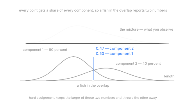
Cut at 20.5 cm and tally, and you've recorded a genuinely ambiguous fish as certain — throwing away what you wanted: how many fish are ambiguous, and how big each group really is.

Two ideas first. A normal distribution is the bell-shaped rule for where measurements fall, set by a centre and a width (the family). Likelihood is how probable your lengths are under a guess at those numbers, and fitting maximises it (the method).

Think of It Like This

Two spray cans on a fence

Someone stood at a fence with two cans of paint. Pick a can, spray one dot, pick again, spray again — nine hundred times, choosing the first can twice as often. Each can throws an oval of mist, dense at the centre, and the ovals overlap in the middle.

You arrive after they've gone. From the dots alone you can work out roughly where each can was held, how wide and tilted its oval was, and how often each was picked.

Now pick a dot from the overlap and ask which can made it. Nobody can. What you get is the odds: it sits where the first can's mist is slightly denser, so it's a little more likely from that one. Fifty-three, forty-seven.

That's the honest answer. Saying "can one" throws away the near coin flip — and the paint has no idea it came from a can at all. The story is something you assumed to explain the fence.

How It Actually Works

The story, then the algorithm

The model is a claim about how your data was made: pick a component with some probability, draw a point from that component's bell curve. Fitting recovers three things per component — its centre, its shape, and how often it gets picked. You can't maximise the likelihood directly, because you'd need to know which component each fish came from, and knowing that needs the components you're fitting. Expectation-maximisation breaks the circle by alternating.

The E step computes, for every fish, the probability it came from each component under the current parameters. Those are the responsibilities, they sum to one per fish, and they are the soft assignment. The M step re-estimates each component's centre, shape, and weight as an average over all 900 fish, weighted by those responsibilities — a fish at 0.53 and 0.47 feeds both.

Repeat. The likelihood rises or holds every iteration and never falls, so it converges. To a local maximum, so restarts matter exactly as they do for k-means.

Not fuzzy k-means

The relationship is exact, not a loose analogy. Force every component spherical and the same width, force the weights equal, then replace each fish's responsibilities with a 1 for the largest and 0 for the rest — the two steps are now k-means.

What you gain is what you stop forcing. Each component carries a full covariance matrix, so it can be elongated and tilted: one year-class might vary a lot in length and little in girth, running diagonally through the space, and a mixture handles that while k-means cuts it up. Weights can differ too, so a group holding a third of the fish isn't pushed to grow. And responsibilities are real output: aggregate them for an expected count per group, fractional fish included.

The dials that matter

Covariance type is the capacity knob. full gives each component its own tilt and stretch, at a parameter cost quadratic in the column count. diagonal allows different widths per column but no tilt. spherical is one width. tied shares one matrix. With forty columns and eight hundred rows, full overfits and diagonal is usually right.

Choosing k is better here than in k-means because you have a likelihood, so you can compare across k with a criterion that charges for parameters — BIC and AIC both do. Fit k from 1 to 8, plot BIC, take the minimum. Still a heuristic, still assuming bell curves, but it beats squinting at an elbow.

Show Me the Code

EM on 900 herring lengths, two components, from a deliberately bad start.

1import numpy as np2
3def em(x: np.ndarray, k: int, steps: int = 80) -> tuple[np.ndarray, np.ndarray, np.ndarray]:4    mu = np.linspace(x.min(), x.max(), k)5    var, w = np.full(k, x.var()), np.full(k, 1.0 / k)6    for _ in range(steps):7        d = w * np.exp(-((x[:, None] - mu) ** 2) / (2 * var)) / np.sqrt(2 * np.pi * var)8        r = d / d.sum(axis=1, keepdims=True)          # E step: one soft membership per fish9        n = r.sum(axis=0)10        mu = (r * x[:, None]).sum(axis=0) / n         # M step: membership-weighted estimates11        var = (r * (x[:, None] - mu) ** 2).sum(axis=0) / n + 1e-6   # the floor stops collapse12        w = n / len(x)13    return mu, np.sqrt(var), w14
15rng = np.random.default_rng(2)16lengths = np.concatenate([rng.normal(17.5, 1.4, 600), rng.normal(24.0, 2.0, 300)])17mu, sd, w = em(lengths, 2)18p = w * np.exp(-((20.5 - mu) ** 2) / (2 * sd ** 2)) / (sd * np.sqrt(2 * np.pi))19print("means", np.round(mu, 2), " weights", np.round(w, 2), " 20.5cm", np.round(p / p.sum(), 2))20# -> means [17.41 24.03]  weights [0.67 0.33]  20.5cm [0.53 0.47]

It recovered 17.5, 24.0 and the two-thirds split from lengths alone. The 20.5 cm fish comes back 0.53 and 0.47 — "we don't know", written down properly.

Watch Out For

A component collapsing onto a handful of points

The log-likelihood climbs, then shoots up absurdly, and the fit is nonsense. Look at the components: one has eleven members and a variance near zero. That's collapse. A bell curve narrowing onto a few near-identical points sends its density there to infinity, and the likelihood with it — the optimiser is doing what you asked.

The fix is a floor. Add a small constant to the covariance diagonal — reg_covar in most libraries, the + 1e-6 above — and drop components whose weight falls under a percent. If it recurs with full covariance, switch to diagonal.

Reading responsibilities as real-world probabilities

A report says a fish has a 53 percent chance of being a young fish. It doesn't. It has a 0.53 responsibility for component one under a model that assumed herring lengths are a sum of two bell curves. If real lengths are skewed, or there are three year-classes, that number is precise and wrong.

Test the assumption rather than trusting the output. Check whether each component's members look normal, refit with k one higher and see whether the split survives, and where you have ground truth — a few hundred fish aged from their ear bones — check whether things called 0.7 land that way about seventy percent of the time.

The Quick Version

Each point came from one of k bell curves, picked with some probability. Fitting recovers each curve's centre, shape, and weight.
EM alternates: the E step gives every point a probability of belonging to each component, the M step re-estimates parameters weighted by those.
Likelihood never falls across iterations, so it converges — to a local maximum, so restart it.
K-means is the special case: spherical equal-width components, equal weights, responsibilities hardened to the nearest.
Full covariance buys tilted elongated clusters; soft assignment buys per-point uncertainty you can aggregate. A real likelihood lets you compare k using BIC.
Guard against collapse with a covariance floor, and don't read responsibilities as real-world probabilities.