Core ML

Clustering Evaluation

There is no answer key, so every score you can compute encodes somebody's definition of a cluster and quietly rewards whichever algorithm happens to share it.

Silhouette rewards compact round groups, so it scores a wrong straight cut through two crescents higher than the correct crescent-shaped grouping

Why Does This Exist?

A 600-hectare farm has 4,000 soil samples on a grid — pH, organic matter, clay fraction, moisture. Cluster them into management zones and the fertiliser spreader can vary its rate as it drives. Then somebody asks the obvious question: is this clustering any good?

With a classifier you'd check the answers. Here there are none. Nobody wrote down the true zone for each sample, and if they had you wouldn't be clustering.

So every measurement is indirect, and each one has a built-in idea of what a cluster looks like. Score a result with a metric that shares your algorithm's assumptions and it approves of itself. If model evaluation is about not fooling yourself with a number, this is the version where the number has an opinion.

Think of It Like This

Testing parts by dropping them through a round hole

A workshop checks its output by dropping every finished part through a 40 mm circular hole. Parts that fall through pass. It's fast, it needs no judgement, and within a year everyone calls it the quality test.

Then the shop starts making brackets. A perfectly machined bracket won't go through, so it fails. Nothing is wrong with the bracket and nothing is wrong with the hole. The hole only ever measured roundness, and somebody read roundness as quality.

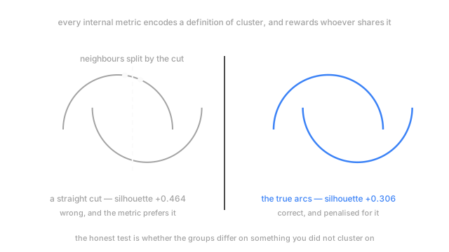
That's silhouette scoring a crescent. It isn't broken — it's answering the question it was built for, which is whether the groups are compact and well separated, and a correct crescent is neither.

There's a second test the workshop never runs: hand the same batch to a different shift and see whether the same parts come back. If the output moves with who's on duty, the process isn't a process.

How It Actually Works

Three families, and they answer three different questions.

Internal: only the data you clustered

Silhouette is the one people use. For each sample take the mean distance to others in its own zone, call it $a$ , and the mean distance to samples in the nearest other zone, call it $b$ :

s = \frac{b - a}{\max(a, b)}

It runs from minus one to one. Near one, the sample sits comfortably inside its own zone; near zero, it's on a boundary; negative, it would be happier elsewhere. Average over all 4,000 for the clustering's score.

Calinski-Harabasz is a ratio of between-cluster to within-cluster variance, so bigger is better and it has no fixed range. Davies-Bouldin averages each cluster's similarity to whichever cluster it most resembles — smaller is better.

Now the catch. All three are built from distances to cluster centres or averages of pairwise distances, so all three are maximised by compact, round, well-separated blobs. Score DBSCAN's crescent zones with silhouette and you penalise it for being correct.

External: labels you happened to have

Sometimes you do have labels — last year's zones, hand-drawn by an agronomist. The adjusted Rand index counts pairs of samples both groupings agree about, together or apart, adjusted so a random grouping scores zero rather than something positive. One is perfect agreement. Normalised mutual information asks how much knowing one grouping tells you about the other, zero to one.

Both validate a method on data where you know the answer. Neither judges a clustering you intend to use — if labels exist for the rows you care about, the honest tool is a classifier.

Stability, and the bar that actually matters

The check almost nobody runs. Bootstrap-resample your 4,000 samples, or split them in half, recluster, and measure whether the same samples keep landing together — an adjusted Rand index between the two runs does it. Repeat thirty times.

A clustering that reshuffles across resamples describes one sample, not the farm. It catches what no internal metric will: k too high, a component that exists because of forty rows, a seed doing the work.

The real bar is downstream, though. A clustering is good if it supports a decision, so here's the test that settles it: do the zones differ on something you didn't cluster on? Pull last season's yield map, never an input, and check whether zone means differ by more than the noise. If they don't, you have a tidy partition of nothing.

Show Me the Code

Two interlocking crescent zones following a drainage channel, scored against a straight left-right cut.

1import numpy as np2
3def silhouette(X: np.ndarray, lab: np.ndarray) -> float:4    D = np.sqrt(((X[:, None] - X[None]) ** 2).sum(-1))5    s = np.empty(len(X))6    for i in range(len(X)):7        own = lab == lab[i]8        a = D[i, own].sum() / max(own.sum() - 1, 1)      # mean distance inside its own group9        b = min(D[i, lab == c].mean() for c in set(lab) - {lab[i]})10        s[i] = (b - a) / max(a, b)11    return float(s.mean())12
13t = np.linspace(0.0, np.pi, 200)14upper = np.column_stack([3 * np.cos(t), 3 * np.sin(t)])15lower = np.column_stack([3 * np.cos(t) + 1.6, -3 * np.sin(t) + 1.2])   # interlocking arcs16X = np.vstack([upper, lower])17zones = np.repeat([0, 1], 200)18cut = (X[:, 0] > X[:, 0].mean()).astype(int)             # a straight left/right split instead19print(f"the two real arcs {silhouette(X, zones):+.3f}   a left/right cut {silhouette(X, cut):+.3f}")20# -> the two real arcs +0.306   a left/right cut +0.464

The wrong answer wins by 0.16, and it isn't close. Maximise silhouette on data like this and you ship the straight cut every time.

Watch Out For

Choosing k by maximising silhouette

The loop looks responsible: fit k from 2 to 12, compute silhouette, take the best. Then the zones come back as two enormous round blobs when the field visibly has four elongated drainage-following strips, and the four-zone solution scored lower.

That's the metric preferring its own shape, not a discovery about the field. Plot silhouette across k next to a stability curve and the BIC from a mixture model, and pay attention to where they disagree. Then pick k for a reason you can say out loud. "Four, because the spreader has four rate settings" beats "five, because 0.41 beat 0.39".

Validating on labels that won't exist in production

You have last year's hand-drawn zones for two fields, score an adjusted Rand index of 0.93 against them, and ship the method across all forty. The score was real. What it measured was that the agronomist's zones were clusterable — that a distance-based method can recover boundaries somebody drew using the same soil properties.

It says nothing about the thirty-eight fields nobody has drawn. Treat an external score as a quick check on the pipeline and nothing more, then validate where you'll deploy: stability across resamples, plus a difference in something you didn't cluster on. And if labels exist everywhere you need them, stop clustering and train a classifier.

The Quick Version

No answer key, so every score is indirect and carries an assumption about cluster shape.
Internal metrics use only the data. Silhouette compares each point's own-cluster distance to its nearest-other-cluster distance, minus one to one; Calinski-Harabasz is a variance ratio you want large; Davies-Bouldin a ratio you want small.
All three reward compact round clusters, so they punish density-based methods for finding correct non-round ones.
External metrics need labels. Adjusted Rand counts agreeing pairs with chance removed; normalised mutual information measures shared information. Both validate a method, not a deployment.
Stability is the underused check: recluster on resamples, see whether the same points stay together.
The bar that counts is whether the clusters differ on something you left out.